Data, Database, Lab Notebook, Recipe and Script
This chapter fully describes every data-handling layer of the Mikrofab semiconductor / TFT / PV measurement and analysis software: the SQLite database that stores measurement summaries and the Data & Search panel that filters it, the sample-centric Lab Notebook (Journal / ELN), the Recipe tools that generate automated measurement sequences, headless operation together with the local REST API, the Python Script / Console workspace, and finally presets / configuration / favorites / user modes. The goal is to let you manage the entire data flow — from a single measurement to an archive of hundreds, and from there to overnight automation and remote control.
Vds/Vgs/Ids/Igs values of every point) are always kept on the file system (CSV / TXT / XLSX / HDF5 / JSON); only a summary (metadata + extracted metrics + the path of the related file) is written to the database. This keeps the database small and fast, so questions like "across 100+ measurements, which TFT has the highest Ion/Ioff?" are answered instantly.The job is not finished once you take a measurement: you need to store that data safely, find it again months later and replot it, query which device performed best, and have the same test repeat itself overnight. This chapter explains the software's "record-keeping and automation" side: the database that shelves measurements like a library, the lab notebook that keeps a sample's fabrication story, self-running recipes, and the headless mode that does the work via commands without opening a screen.
- Why it is done: to turn individual measurements into a searchable, non-losing archive and into automation that runs without a human at the keyboard.
- What it teaches / measures: where and how data is stored, how it is filtered and compared, and how it is generated automatically.
- Where it is used: research, quality control and long-term stability studies where many devices are measured.
1. Overview of the Data Architecture
The software manages user data across three separate SQLite databases plus raw outputs distributed on the file system. All of them live under your user-data root (user_data_root) and none are written to the installation directory.
| Store | File | Content | Access layer |
|---|---|---|---|
| Measurement summary DB | measurements.db | A summary of every completed measurement + analysis results | MeasurementDatabase |
| Lab Notebook DB | journal.db | Sample headers + process-step cards | JournalDatabase |
| Raw measurement files | measurements/<run-folder>/… | CSV / TXT / XLSX / JSON / HDF5 / report | DataWriter |
| Attachments | journal/sample_<id>/attachments/ | Images attached to a sample | file system |
| Configuration | config/user_config.json | User settings, view profiles | ConfigManager |
| Presets | presets/<panel>/<name>.json | Named parameter sets | PresetManager |
All databases conform to the same database standard: single-gateway data access (all queries parameterized — no SQL injection), schema versioning + forward migration (automatic backup before migration), append-only + soft-delete (deleted_at), a full audit trail (audit_log), WAL journal mode, and the backup() / check_integrity() maintenance functions.
2. Measurement Database (measurements.db)
The measurement database is a small, fast ledger that keeps a summary of every completed measurement like a library catalog card. All of the raw numbers stay in files; only a "who, when, which mode, which result" summary and the path of the related file are written to the database. This lets you search and sort across hundreds of measurements within seconds.
- Why it is done: to answer questions like "which TFT has the highest Ion/Ioff?" without opening hundreds of files one by one.
- What it teaches / measures: it shows each measurement's extracted metrics (Vth, mobility, SS, On/Off …) together with its context (geometry, device, time).
- Where it is used: finding the best device in multi-measurement archives, comparing results and reporting.
2.1 Which fields are written?
When a measurement completes successfully and its files are saved, the software automatically adds a summary row (MeasurementDatabase.record). Geometry and measurement conditions, all extracted metrics and the device identity fall into this row; in addition, anything without a corresponding schema column is stored as a full capture in the params_json / summary_json columns (no data is lost).
Identifier and context fields
| Column | Type | Description |
|---|---|---|
id | INTEGER | Auto primary key |
recorded_at | TEXT | Time recorded (local ISO) |
started_at | TEXT | Measurement start time |
tft_id | TEXT | Sample / device identifier (Lab Notebook bridge) |
mode | TEXT | Measurement mode (TRANSFER, IV, DIODE, PV_JV …) |
software_version | TEXT | Software version that took the measurement |
point_count | INTEGER | Total number of data points |
csv_path | TEXT | Path of the related raw CSV file (loaded by double-click) |
user_comment / note | TEXT | User comment / analysis note |
TFT / On-Off metrics (Transfer mode)
| Column | Unit | Description |
|---|---|---|
ion, ioff | A | On / off state current |
ion_ioff | — | On/off ratio |
ion_ioff_robust, ioff_robust, ioff_std | —, A, A | Robust Ioff estimate + scatter |
vth | V | Threshold voltage (method via extraction_method) |
vth_y_v, mu0_y_cm2_vs, y_r2 | V, cm²/Vs, — | Y-function method results |
mu_fe | cm²/Vs | Field-effect mobility |
ss | mV/dec | Subthreshold swing |
ss_r2 | — | SS linear fit quality |
gm_max, gm_max_vgs | S, V | Maximum transconductance + the Vgs at which it occurs |
dit_cm2_ev | cm⁻²eV⁻¹ | Interface trap density |
vth_fwd_v, vth_bwd_v, delta_vth_v | V | Forward/backward Vth + hysteresis shift |
hysteresis_window_v | V | Hysteresis window |
Output (IV / Output) metrics
| Column | Unit | Description |
|---|---|---|
ron_ohm | Ω | On-state resistance |
output_resistance_ohm | Ω | Output resistance (rₒ) |
lambda_per_v | 1/V | Channel-length modulation (λ) |
vth_sat_v, mu_sat_cm2_vs, mu_sat_r2 | V, cm²/Vs, — | Vth / mobility from saturation |
Diode / Schottky metrics
| Column | Unit | Description |
|---|---|---|
forward_current | A | Forward current |
reverse_leakage | A | Reverse leakage current |
turn_on_voltage | V | Turn-on voltage |
rectification_ratio | — | Rectification ratio |
series_resistance_ohm | Ω | Series resistance |
ideality_factor | — | Ideality factor (n) |
Geometry and device conditions: w_um, l_um (µm), cox_nf_cm2 (nF/cm²), nplc, averages, sweep_direction, keithley_idn, visa_resource, drain_channel, gate_channel, relay_enabled.
µ_sat = (2L / (W·Cox)) · (∂√Ids/∂Vgs)² and lands in the mu_sat_cm2_vs column; the associated fit quality goes into mu_sat_r2. The database only stores and searches these values.2.2 Schema version, migration and durability
The database schema is versioned (schema_version); the current version is 4. An old database is upgraded to the latest version in a single step on first open without losing data (v1 → v2 → v3 → v4). The migration steps:
- v1 → v2: Soft-delete column (
deleted_at) +audit_logtable + indexes. - v2 → v3: All collected/computed metric columns (the tables above) + the
params_json/summary_jsonfull-capture columns. - v3 → v4: A separate
analysis_resultstable for analysis results.
db_backups/measurements.pre_migration_vN.<time>.db). Thanks to WAL (Write-Ahead Logging) journal mode, records stay consistent even if the application crashes.2.3 Data & Search Panel — filtering, sorting, column selector
This panel is a screen that queries the database live, a cross between a search engine and a spreadsheet: with sample/mode filters, free-text search and sorting by metric, you quickly find the record you are after. You can choose which columns appear and save that layout as a "view profile".
- Why it is done: to instantly sift through a large pile of measurements and surface the best/relevant records.
- What it teaches / measures: it presents records as a sorted, comparable table by the metric you choose (e.g. Ion/Ioff, µFE).
- Where it is used: device screening, batch comparison and quick quality-control sweeps.
The panel in the data workspace (DatabasePanel) queries the database live. At the top there are three filters + one sort control:
| Control | Function |
|---|---|
| TFT dropdown | Only records of the selected sample/device (auto-populated from the database) |
| Mode dropdown | Only the selected measurement mode |
| Search box | Free text; LIKE search within user_comment, note and csv_path |
| Sort dropdown | Database query order (table below) |
The top "Sort" list determines the query's ORDER BY order; empty (NULL) values are always pushed to the end, so empty rows do not float to the top in "highest metric" queries:
| Label | Column | Direction |
|---|---|---|
| Date | recorded_at | Descending |
| Ion/Ioff | ion_ioff | Descending |
| µFE | mu_fe | Descending |
| SS | ss | Ascending (smaller is better) |
| Vth | vth | Ascending |
| Ron | ron_ohm | Ascending |
| µ_sat | mu_sat_cm2_vs | Descending |
| Point count | point_count | Descending |
Two-tier sorting: In addition to the query order, you can click any column header to re-sort the loaded rows client-side by that value (numeric/textual). Numeric columns are sorted as true numbers, including text such as "3.832e+05".
Column selector and view profiles: With the "Columns…" button (or the header right-click menu) you choose which columns are shown and their order. Columns are moved by drag-and-drop or with the To Top / Up / Down / To Bottom buttons. You can save a layout as a named view profile; a profile stores not only the columns but also the top sort selection and the filters — when selected, all of them are restored together. The selection is written to the configuration (db_view_profiles, db_visible_columns, db_column_order, db_active_profile).
2.4 Loading a result into the plot by double-click
When you double-click a table row, the raw measurement file at that record's csv_path field is opened via a signal (file_activated) and reloaded into the measurement plot — the curve is redrawn. This lets you visually review a sweep taken weeks ago with a single click. File reading is done with DataWriter.read_points_csv (columns map exactly).
csv_path is populated. If you leave this field empty in manually added records, double-click does nothing; you can enter a file path by hand if you wish.2.5 Manual add / edit / delete / undo
The panel is not read-only; all write operations pass through the data-access layer and are written to the audit trail:
- Add: Opens a blank form; numeric fields are parsed, empty ones become
None. Ifrecorded_atis empty it is assigned automatically (add_manual, audit:create). - Edit: Opens the selected record in the same form; only whitelisted columns are written, and the previous state is recorded to the audit trail via
before_json(update_measurement). - Delete (soft): The default deletion. The record is marked with
deleted_at, hidden from queries but its data remains (soft_delete). With Ctrl/Shift you can multi-select and delete in bulk. - Undo: Restores a soft-deleted record (
restore). - Hard Delete: Exceptional; first takes an automatic file backup, then deletes the row entirely (
hard_delete, audit mandatory). - Show deleted checkbox: when ticked, soft-deleted records appear grayed out and struck through.
2.6 Analysis results table (analysis_results)
This separate table, introduced with schema v4, holds the results produced by the Analysis chapter (oscilloscope I-t / V-t, spectral, noise, PV metrics, etc.). Columns: recorded_at, title, analysis_type, source_file, source_kind, tft_id, user_comment, note, point_count, result_json, series_json, params_json. Computed results and parameters are stored in JSON columns; listing/filtering is done by analysis_type, tft_id and free text (list_analyses). It shares the same soft-delete + audit pattern as the measurement table.
3. Sample Journal (Lab Notebook / ELN)
The Lab Notebook is a digital sample dossier that keeps each sample's full history, from fabrication to measurement, as cards. It gathers every step — cleaning, thin-film, lithography, annealing — along with its photographs and the resulting measurements under a single sample.
- Why it is done: to answer "why did this device turn out this way?" by relating fabrication steps to results.
- What it teaches / measures: it shows a sample's process history and the electrical results bound to it (the
tft_idbridge) in one place. - Where it is used: process development, reproducibility tracking and traceable/accredited laboratory records.
The Lab Notebook is a sample-centric electronic lab notebook (ELN). When you fabricate a material/sample, you record the fabrication steps (thin-film, lithography, etch, anneal, measurement, note …) as cards, attach images, and link this application's measurements (via the tft_id bridge).
3.1 Two tables: samples + sample_steps
| Table | Row meaning | Key fields |
|---|---|---|
samples | A fabricated sample / wafer / die | sample_id (unique), title, status, operator, facility, batch_lot, parent_wafer_id, substrate_material, active_material, ambient_temp_c, ambient_rh_pct, cleanroom_class, tags, notes |
sample_steps | A process-step card belonging to that sample | ordinal (order), step_type, title, params_json, attachments_json, linked_measurement_id, note |
sample_id is the user-facing identity of the sample and corresponds to the tft_id field of measurements — this is the bridge between the Lab Notebook and the measurement database. Raw images are not in the database but under journal/sample_<id>/attachments/; the database only keeps the path.
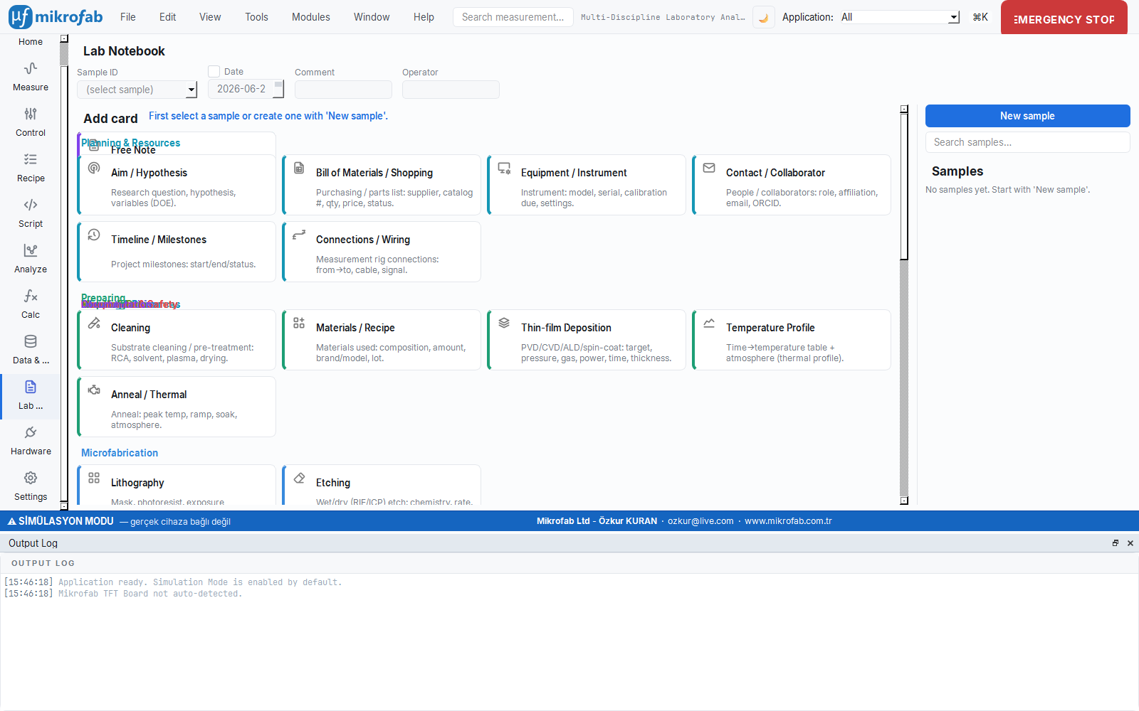
3.2 Quick-add and the combined Sample ID
At the top of the list page there are four fields: Sample ID (type or pick from the list), an optional Date, a Comment and an Operator. These are combined live into a single DB-safe identifier:
For example, with base TFT-ZnO, date enabled, comment rev1 → TFT-ZnO-2026-06-22-rev1. Spaces within parts become _ and invalid characters are dropped. When the Sample ID is empty the gallery cards are disabled; a live preview of the combined identifier (→ …) appears at the top.
3.3 Card gallery and step types
The gallery in the left column consists of clickable cards that are grouped into categories, just like the Measurement page, and wrap to the available width with drag-and-drop (FlowLayout). When you click a card: the sample is found-or-created using the combined identifier, the corresponding step_type card is added, and the sample detail opens.
Supported step (card) types (by category):
| Group | Step types |
|---|---|
| Core process | cleaning, materials, thinfilm, tempprofile, anneal, litho, etch, process, checklist, diagram, measurement, note |
| R&D extension | aim, bom, equipment, contact, timeline, wiring, reference, document, xrd, microscopy, spectroscopy, test, standard, safety, protocol, signoff, result, statistics |
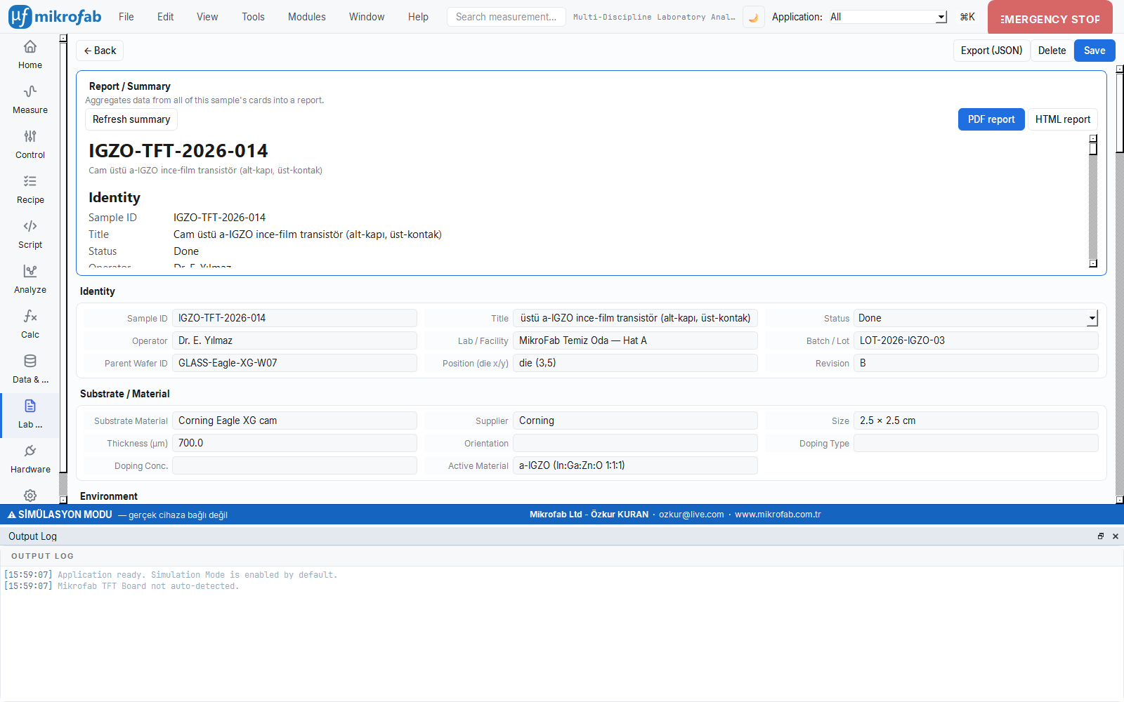
3.4 Sample detail and the measurement bridge
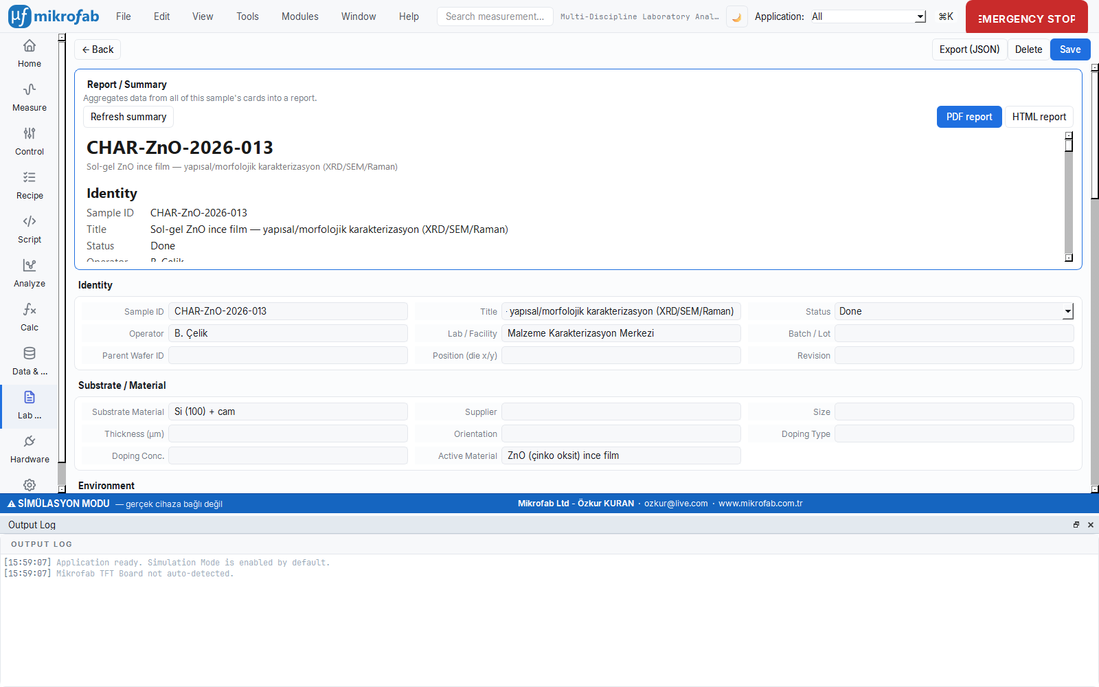
The detail page splits the header fields into logical sections: Identity (sample_id, title, status, operator, facility, batch/lot, parent-wafer, location, revision), Substrate (material, supplier, size, thickness, orientation, doping type/density, active material), Ambient (temperature, relative humidity, cleanroom class) and Notes (tags, free note). Every header change is written to the audit trail. Step cards are arranged in ordinal order in a 1–3 column grid depending on screen width. A measurement card can link a record in the measurement database via linked_measurement_id; this unifies the sample's process history and its electrical results in one place.
UNIQUE indexed; two samples cannot be created with the same identifier. If you soft-delete a sample, its steps are hidden along with it; when restoring you may need to bring the steps back manually.3.5 Example Lab Notebooks — 10 fully populated demo samples
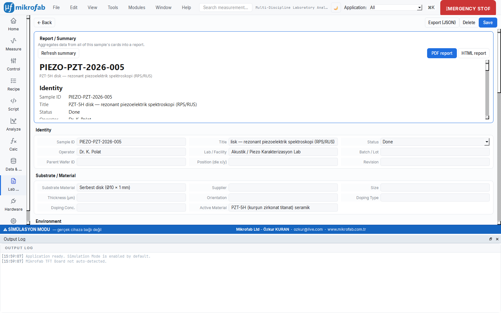
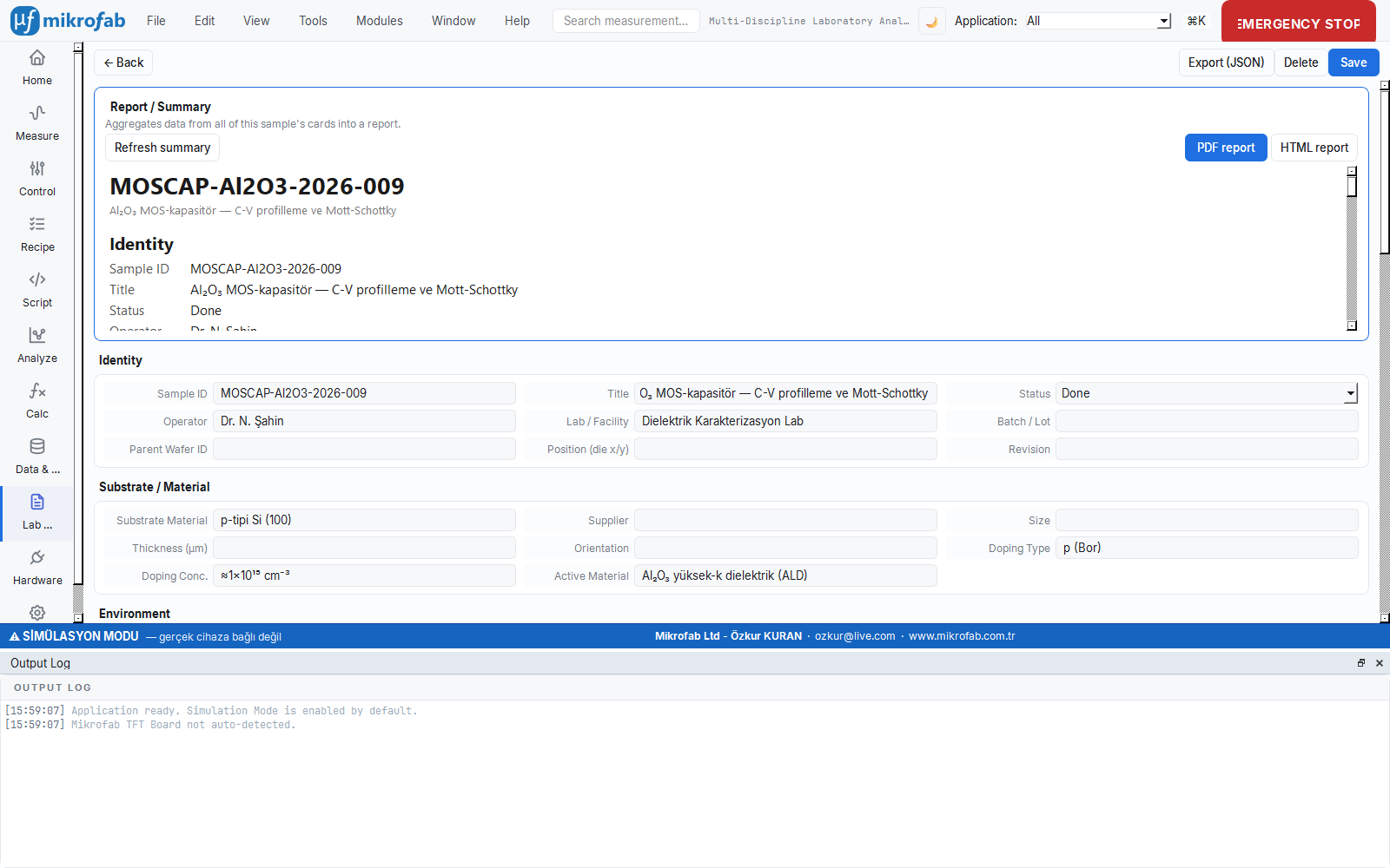
The software ships with an empty Lab Notebook (ELN); however, the value of most features is hard to grasp without seeing "what a full notebook looks like." For this reason, 10 example samples representing ten different work areas are shipped with the application. Each sample follows a real laboratory scenario (microfabrication, project planning, analysis, measurement campaign, solar cell, RRAM, piezoelectric, dielectric, quality/calibration and materials characterization) from start to finish: with process steps, measurement links, result cards and Turkish HTML reports that open with a single click.
These demos are a "teaching showcase": before you fill the notebook yourself, they show what a well-kept electronic lab notebook (ELN) looks like.
- Traceability — substrate/material data sheet, operator, facility, batch-lot and the timestamp of each step bring a sample's entire history together in one place.
- Process-step cards — show with live examples how each card family is filled in: cleaning, thin-film, lithography, etch, temperature profile, measurement, statistics, result, sign-off.
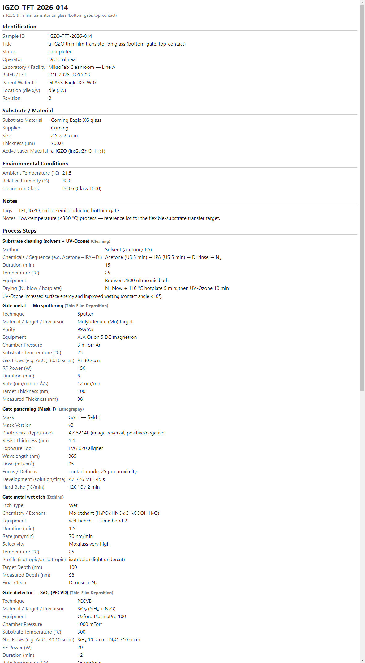
- Result → report chain — shows what the printable/emailable Turkish HTML report, generated from the notebook's data with a single click, looks like.
- Different types of work — not only measurement; examples of how project planning and quality/calibration notebooks are kept with the same tool.
Loading the demo
There are two ways to see the demo live. The application reads Lab Notebook data from the journal.db file in the user-data folder; the demo is a pre-populated copy of that file.
- Back up your own notebook. Copy your existing
journal.dbfile in the user-data folder to a safe place (to restore after the demo). - Copy the demo. Copy the
examples/journal_demo/journal.dbfile into the user-data folder (over the existing one). - Switch to the Lab Notebook workspace. Open the application and switch to the
Lab Notebookarea from the left rail; the 10 example samples are listed in the gallery, and you can click each to inspect its steps and reports. - Restore the backup when done. Copy the backup you took in step 1 back into the user-data folder; your own notebook returns intact.
Alternative (no application): If you only want to see the reports, it is enough to open the HTML files under examples/journal_demo/raporlar/ (or the Open links in this manual) directly in a browser; there is no need to launch the application.
journal.db file; all demo output is written only to the examples/journal_demo/ folder. Since you perform the copy step above yourself, backing up your own notebook before the demo is the only important step.
The ten samples — summary
| Sample ID | Topic | Work area / focus | Status | Steps | Report |
|---|---|---|---|---|---|
IGZO-TFT-2026-014 | a-IGZO thin-film transistor on glass | Microfabrication + measurement (full flow) | ✓ Completed | 11 | Open |
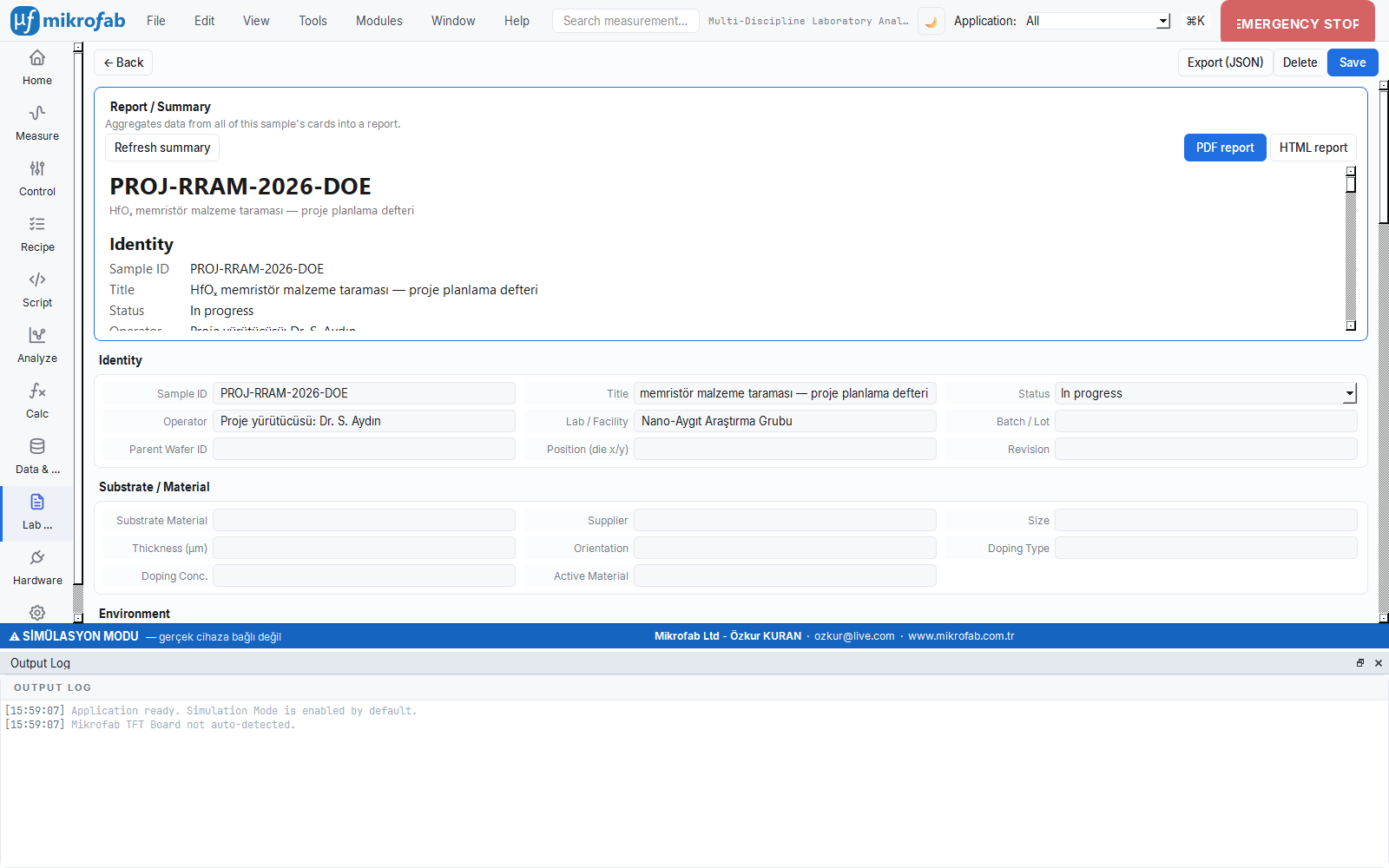
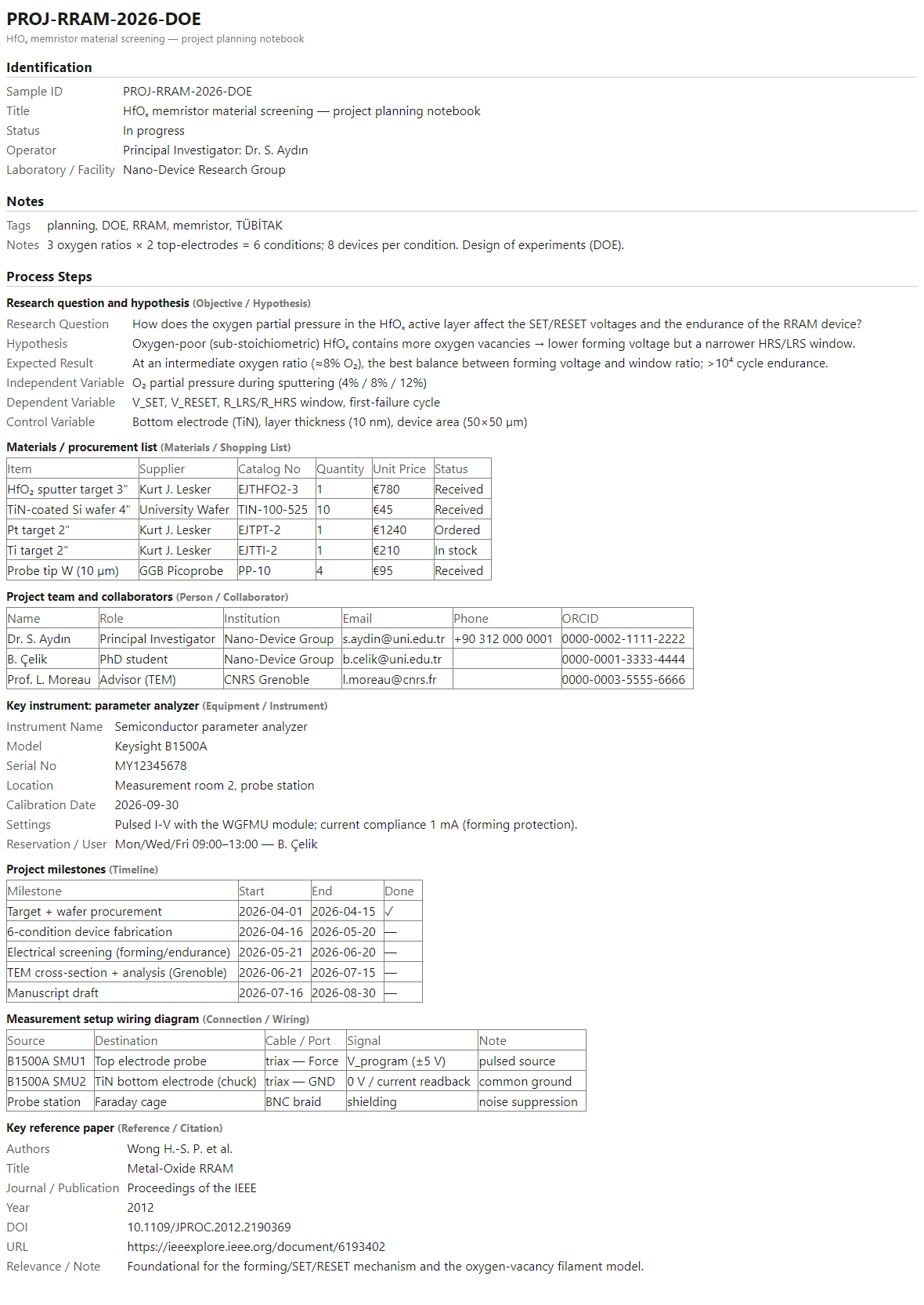
PROJ-RRAM-2026-DOE | HfOₓ memristor material screening | Project planning (DOE) | ⌛ In progress | 7 | Open |
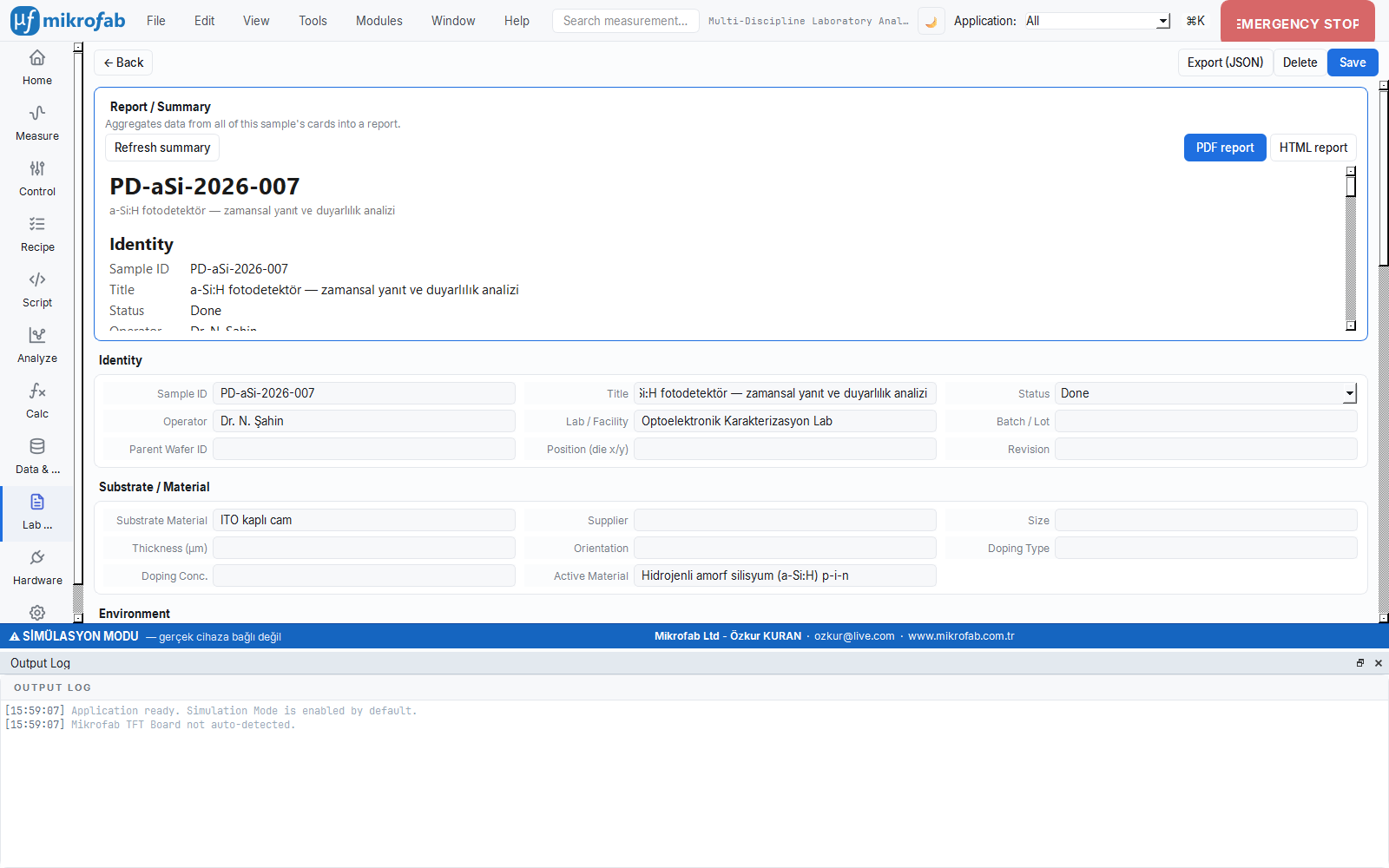
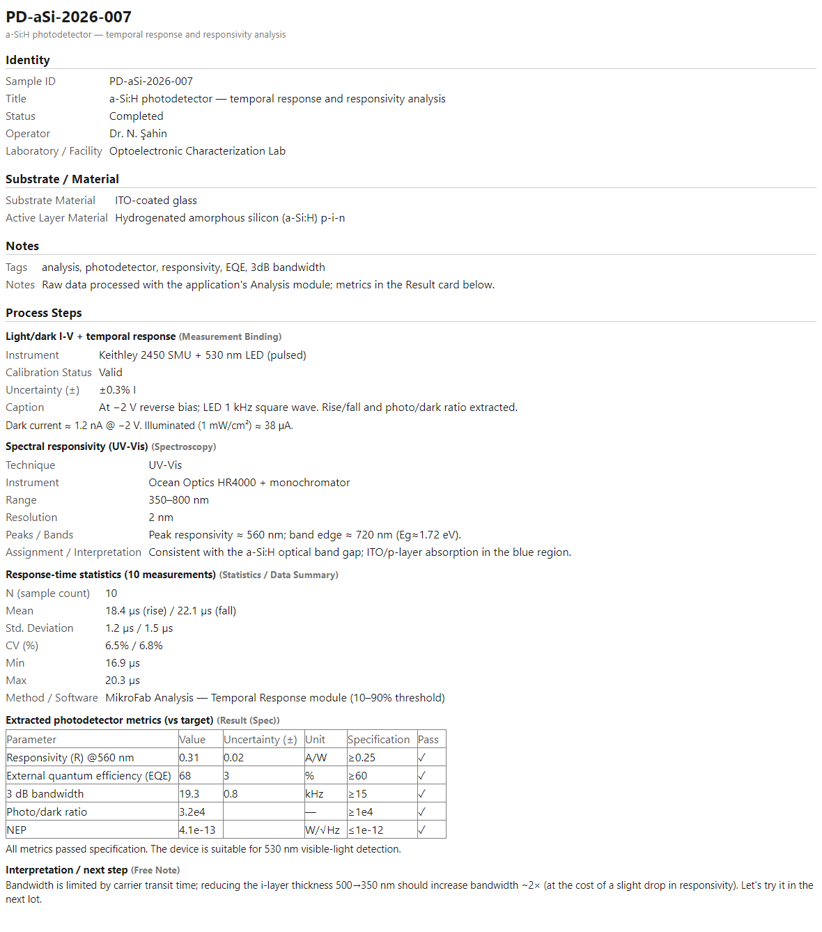
PD-aSi-2026-007 | a-Si:H photodetector | Analysis (responsivity / EQE / band) | ✓ Completed | 5 | Open |
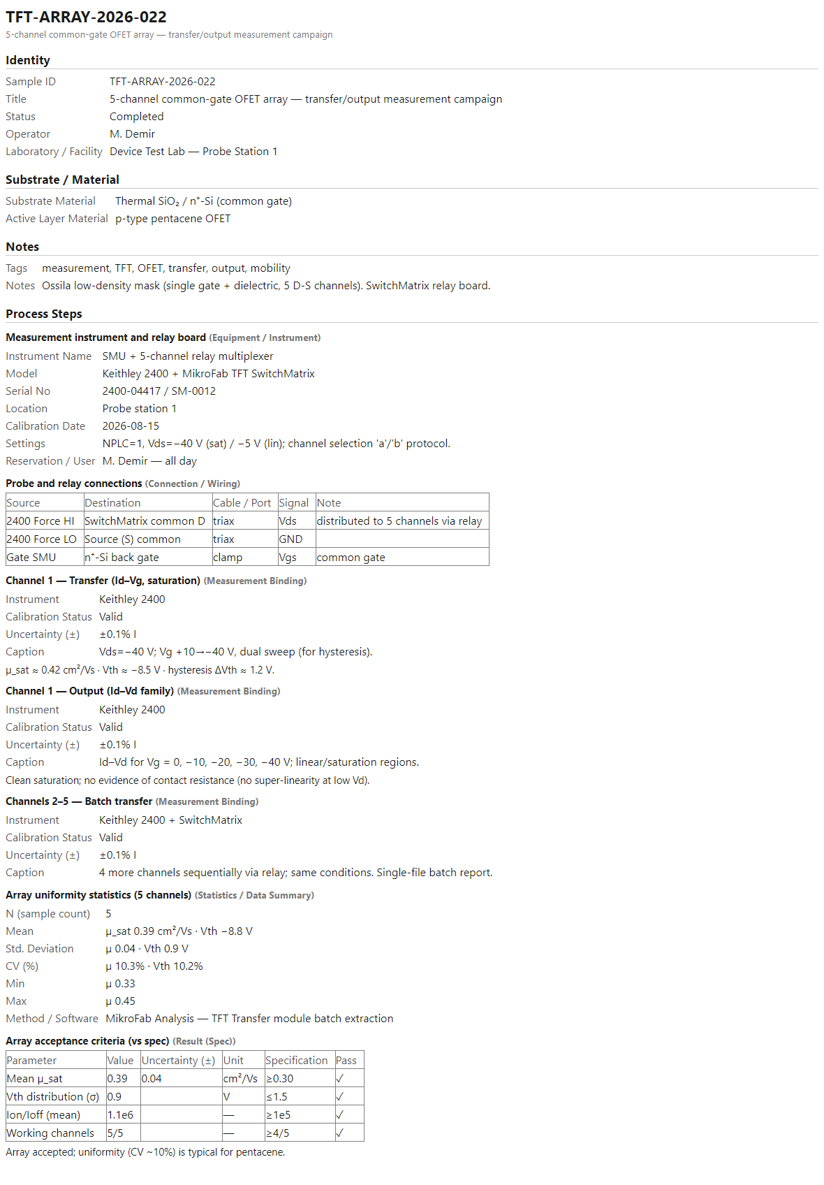
TFT-ARRAY-2026-022 | 5-channel common-gate OFET array | Measurement campaign (transfer/output) | ✓ Completed | 7 | Open |
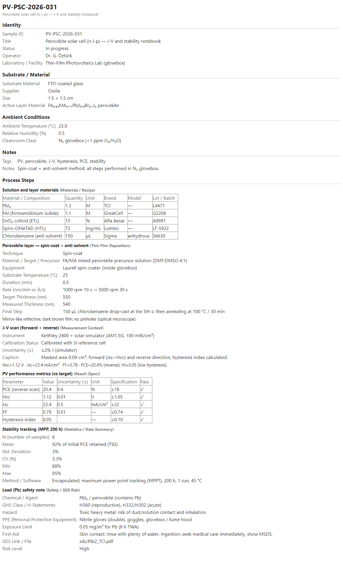
PV-PSC-2026-031 | Perovskite solar cell (n-i-p) | Solar cell (J-V, stability) | ⌛ In progress | 6 | Open |
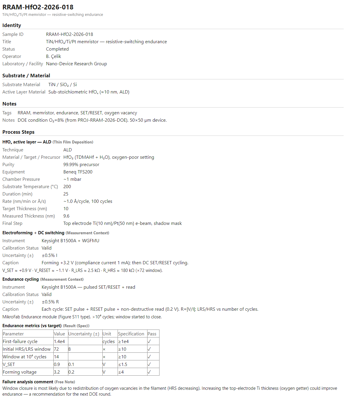
RRAM-HfO2-2026-018 | TiN/HfOₓ/Ti/Pt memristor | RRAM (switching / endurance) | ✓ Completed | 5 | Open |
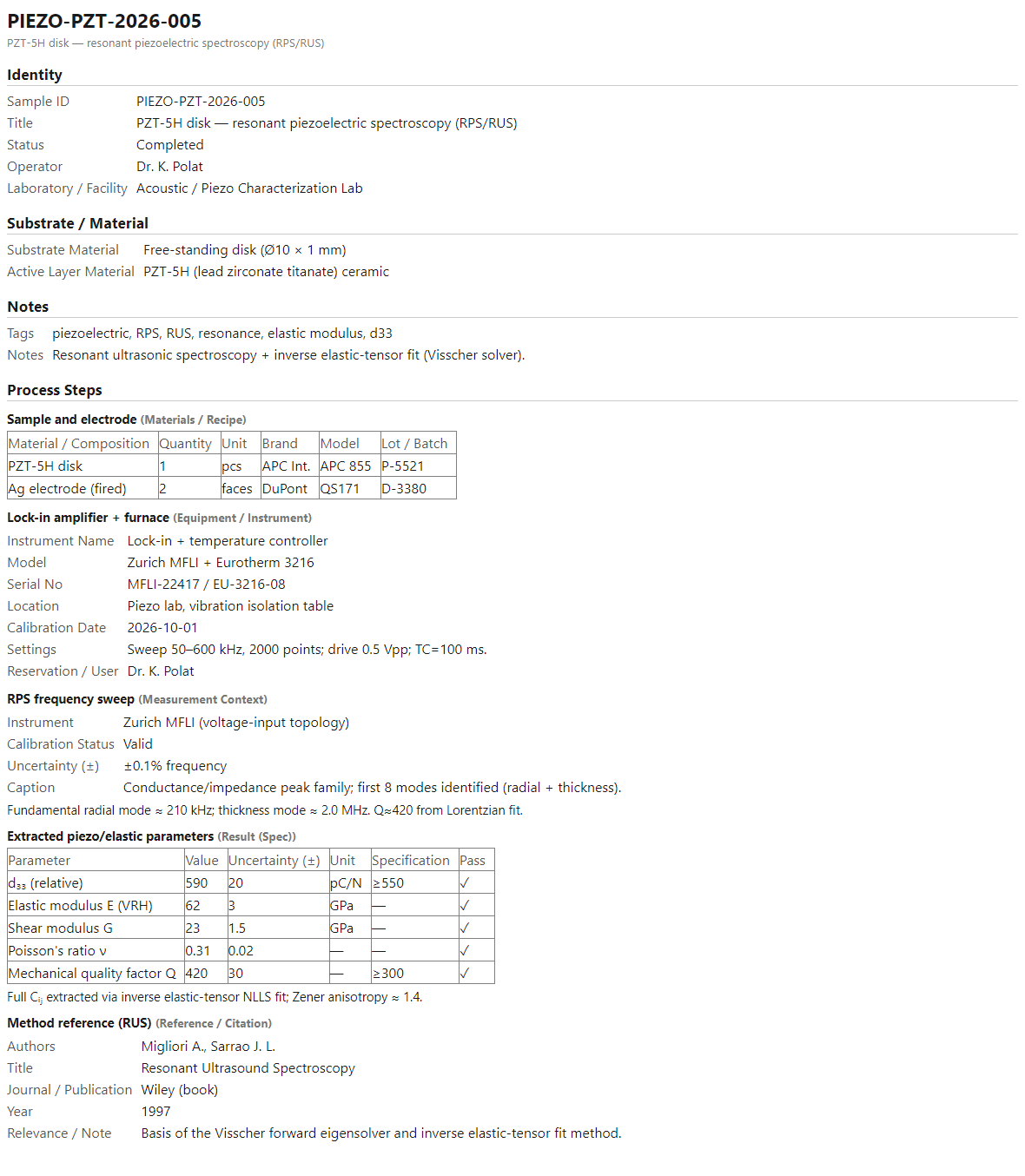
PIEZO-PZT-2026-005 | PZT-5H disk | Piezoelectric (RPS / RUS) | ✓ Completed | 5 | Open |
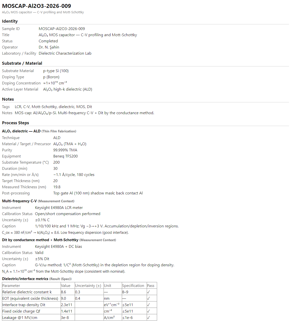
MOSCAP-Al2O3-2026-009 | Al₂O₃ MOS capacitor | Dielectric (C-V / Mott-Schottky) | ✓ Completed | 4 | Open |
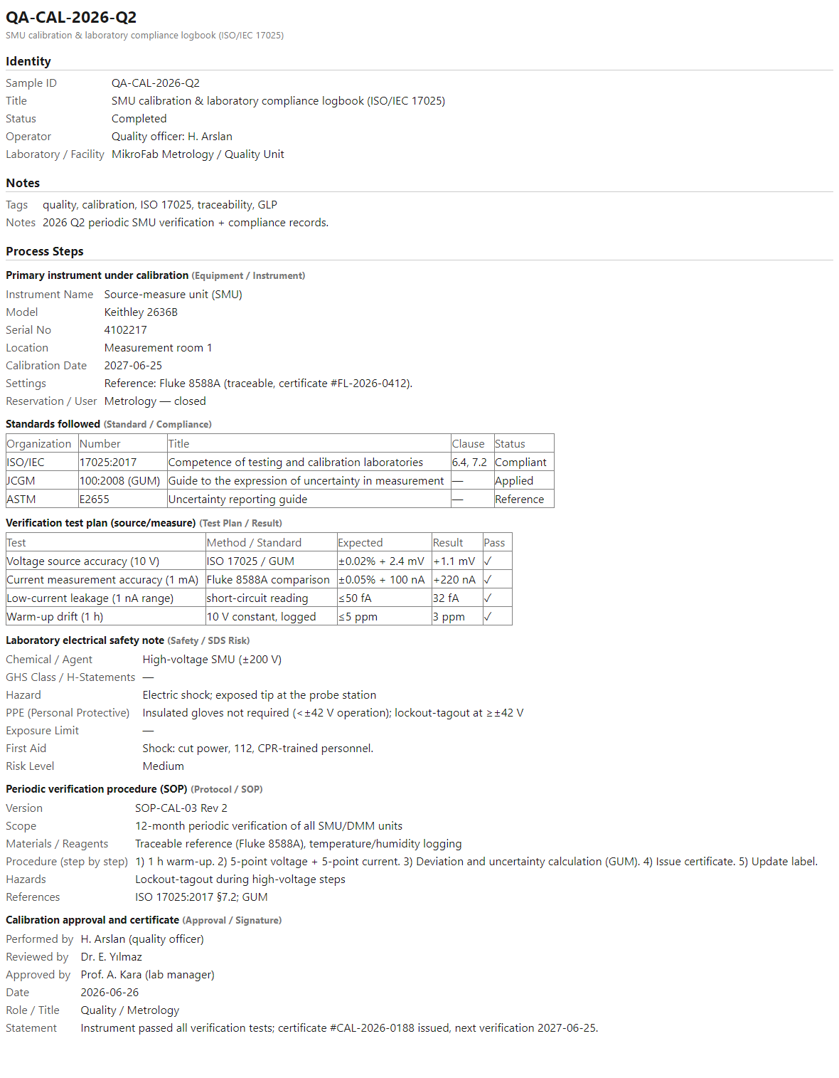
QA-CAL-2026-Q2 | SMU calibration notebook | Quality / calibration (ISO/IEC 17025) | ✓ Completed | 6 | Open |
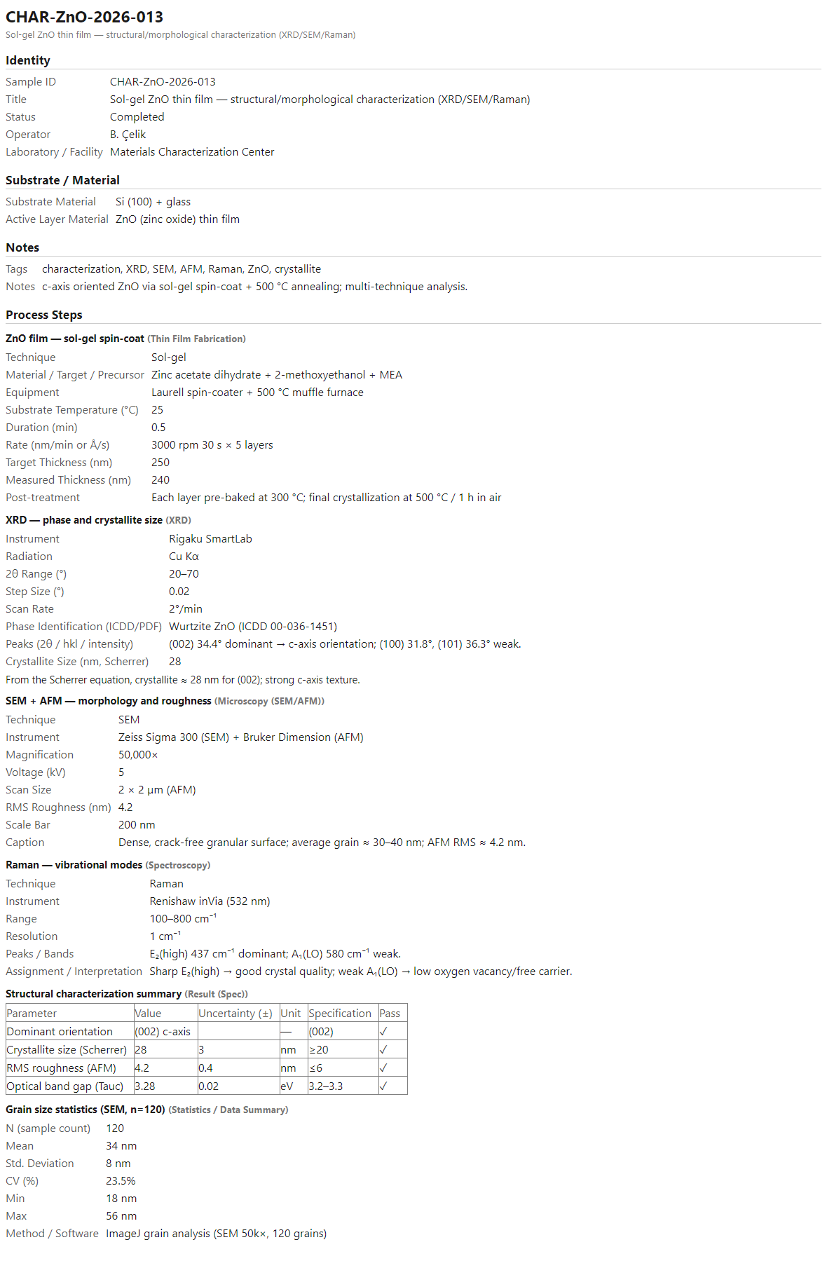
CHAR-ZnO-2026-013 | Sol-gel ZnO thin film | Characterization (XRD / SEM / Raman) | ✓ Completed | 6 | Open |
1. IGZO-TFT-2026-014 — a-IGZO thin-film transistor on glass ✓ Completed
The notebook's "flagship" example: it documents end-to-end, in 11 steps, the from-scratch fabrication and characterization of a bottom-gate / top-contact a-IGZO TFT. The steps follow a complete microfabrication chain: substrate cleaning (solvent + UV-Ozone) → Mo gate metal sputtering → gate patterning (Mask 1) → wet etch → PECVD SiO₂ gate dielectric → a-IGZO active layer sputtering → active island patterning (Mask 2) → e-beam Ti/Au source/drain (W/L = 100/20 µm) → 300 °C / 1 h post-anneal temperature profile → transfer characterization (Id–Vg) → lot closeout sign-off. The low-temperature (≤350 °C) process is kept as a reference lot for transfer to flexible substrates. Key result: µ_sat ≈ 11.4 cm²/Vs, Vth ≈ +0.8 V, SS ≈ 0.18 V/dec and Ion/Ioff ≈ 2×10⁸.
2. PROJ-RRAM-2026-DOE — HfOₓ memristor material screening (planning) ⌛ In progress
This notebook is a project planning example rather than a measurement: it shows that the same ELN tool is also used to document a design of experiments (DOE). 7 steps set up the research flow: research question and hypothesis (aim) → material/purchasing list (bom) → project team and collaborators (contact) → key instrument: parameter analyzer (equipment) → project milestones (timeline) → measurement setup wiring diagram (wiring) → core reference paper (reference). The design is laid out as 3 oxygen ratios × 2 top electrodes = 6 conditions, with 8 devices per condition. Hypothesis: oxygen-poor (sub-stoichiometric) HfOₓ contains more oxygen vacancies → lower forming voltage but a narrower HRS/LRS window; the expected optimum is at a medium oxygen ratio (≈8% O₂). This notebook is the parent plan from which RRAM measurement notebook number 6 below (the O₂ = 8% condition) was born.
3. PD-aSi-2026-007 — a-Si:H photodetector analysis ✓ Completed
An analysis notebook example: the temporal response and responsivity of a p-i-n hydrogenated amorphous silicon (a-Si:H) photodetector on ITO-coated glass are documented in 5 steps, with metrics extracted by the application's Analysis module. The steps: light/dark I-V + temporal response measurement → spectral responsivity (UV-Vis spectroscopy) → response-time statistics (10 measurements) → extracted photodetector metrics (result card against target) → comment / next-step note. Key result: dark current ≈ 1.2 nA @ −2 V, light (1 mW/cm²) current ≈ 38 µA; all metrics passed the specification and the device was found suitable for 530 nm visible-light detection. The next-step note suggests reducing the i-layer thickness from 500→350 nm to roughly double the bandwidth (at the cost of a slight drop in responsivity).
4. TFT-ARRAY-2026-022 — 5-channel common-gate OFET array ✓ Completed
A measurement campaign example: the transfer and output measurements of a p-type pentacene OFET array (single gate + dielectric, 5 source-drain channels, Ossila low-density mask) on a thermal SiO₂ / n⁺-Si common gate are collected in 7 steps. The steps: measurement instrument and relay board (SwitchMatrix) → probe and relay connections → Channel 1 transfer (Id–Vg, saturation) → Channel 1 output (Id–Vd family) → Channels 2–5 batch transfer → array uniformity statistics (5 channels) → array acceptance criteria (against specification). Key result: µ_sat ≈ 0.42 cm²/Vs, Vth ≈ −8.5 V, hysteresis ΔVth ≈ 1.2 V; the output curves show clean saturation (no evidence of contact resistance). The array was accepted; the uniformity (CV ~10%) was found typical for pentacene.
5. PV-PSC-2026-031 — perovskite solar cell (n-i-p) ⌛ In progress
A solar cell (PV) notebook: the J-V performance and stability of an FA₀.₈₃MA₀.₁₇Pb(I₀.₉Br₀.₁)₃ perovskite n-i-p cell on FTO-coated glass are tracked in 6 steps (all processing in an N₂ glovebox). The steps: solution and layer materials (materials) → perovskite layer spin-coat + anti-solvent (thin-film) → J-V scan (forward + reverse) → PV performance metrics (against target) → stability tracking (MPP, 200 h) → lead (Pb) safety note. The film was recorded as "mirror-like reflective, dark brown" and pinhole-free. Key result (reverse scan): Voc = 1.12 V, Jsc = 23.4 mA/cm², FF = 0.78, PCE = 20.4%; hysteresis index HI ≈ 0.05 (low hysteresis). Because stability tracking is ongoing, the notebook is in the "In progress" state.

6. RRAM-HfO2-2026-018 — TiN/HfOₓ/Ti/Pt memristor ✓ Completed
An RRAM / resistive-switching notebook: the switching behavior and endurance of an ≈10 nm sub-stoichiometric HfOₓ (50×50 µm) device grown by ALD — born from the O₂ = 8% condition of DOE plan number 2 — are documented in 5 steps. The steps: HfOₓ active layer — ALD (thin-film) → electroforming + DC switching (forming +3.2 V, current limit 1 mA; Keysight B1500A) → endurance cycling (MikroFab Endurance module) → endurance metrics (against target) → failure-analysis comment. Key result: V_SET ≈ +0.9 V, V_RESET ≈ −1.1 V, R_LRS ≈ 2.5 kΩ, R_HRS ≈ 180 kΩ (×72 window); after >10⁴ cycles the window began to close. The failure analysis attributes the closure to the redistribution of oxygen vacancies in the filament and recommends increasing the top-electrode Ti thickness (oxygen getter) in the next DOE round.
7. PIEZO-PZT-2026-005 — PZT-5H disk (RPS/RUS) ✓ Completed
A piezoelectric characterization notebook: resonant piezoelectric / ultrasonic spectroscopy (RPS/RUS) is carried out on a free PZT-5H ceramic disk (Ø10 × 1 mm) in 5 steps. The steps: sample and electrode (materials) → lock-in amplifier + furnace (equipment) → RPS frequency sweep → extracted piezo/elastic parameters (result) → method reference (RUS). In the sweep, the fundamental radial mode ≈ 210 kHz, the thickness mode ≈ 2.0 MHz; a Lorentzian fit yielded Q ≈ 420. The full elastic tensor Cᵢⱼ was extracted via an inverse elastic-tensor NLLS fit (Visscher solver). Key result: d₃₃ (relative) 590 ± 20 pC/N (≥550 ✓), elastic modulus E (VRH) 62 ± 3 GPa, shear modulus G 23 ± 1.5 GPa, Poisson's ratio ν 0.31, mechanical quality factor Q 420 (≥300 ✓); Zener anisotropy ≈ 1.4. The method is based on the RUS work of Migliori & Sarrao.
8. MOSCAP-Al2O3-2026-009 — Al₂O₃ MOS capacitor ✓ Completed
A dielectric characterization notebook: C-V profiling and Mott-Schottky analysis of an Al/Al₂O₃/p-Si MOS capacitor with an ALD Al₂O₃ high-k dielectric on p-type Si (100) are documented in 4 steps. The steps: Al₂O₃ dielectric — ALD (thin-film) → multi-frequency C-V (1 kHz, 10 kHz, 100 kHz and 1 MHz; Vg −3→+3 V) → Dit by the conductance method + Mott-Schottky → dielectric/interface metrics (result). Key result: C_ox ≈ 380 nF/cm² → k(Al₂O₃) ≈ 8.6 (low frequency dispersion, good interface), EOT ≈ 9.0 nm, interface trap density Dit ≈ 2.3×10¹¹ eV⁻¹cm⁻² (≤5×10¹¹ ✓), and from the Mott-Schottky slope a doping density N_A ≈ 1.1×10¹⁵ cm⁻³ (consistent with the nominal value).
9. QA-CAL-2026-Q2 — SMU calibration notebook (ISO/IEC 17025) ✓ Completed
A quality / calibration notebook: it shows that the ELN can hold not only device records but also laboratory compliance records. The periodic SMU verification for Q2 2026 is documented in 6 steps. The steps: the primary instrument being calibrated (equipment) → the standards followed (standard) → verification test plan: source/measure (test) → laboratory electrical safety note (safety) → periodic verification procedure/SOP (protocol) → calibration sign-off and certificate (signoff). A traceable Fluke 8588A (certificate #FL-2026-0412) was used as the reference; the standards followed are ISO/IEC 17025, JCGM 100:2008 (GUM) and ASTM E2655. Key result: the instrument passed all verification tests; certificate #CAL-2026-0188 was issued, with the next verification date 2027-06-25.

10. CHAR-ZnO-2026-013 — sol-gel ZnO thin-film characterization ✓ Completed
A multi-technique materials characterization notebook: the structural and morphological analysis of a c-axis oriented ZnO thin film grown by sol-gel spin-coat + 500 °C anneal on Si (100) and glass is collected in 6 steps. The steps: ZnO film — sol-gel spin-coat (thin-film) → XRD: phase and crystallite size → SEM + AFM: morphology and roughness → Raman: vibrational modes → structural characterization summary (result) → grain-size statistics (SEM, n=120). Key result: a strong (002) c-axis texture in XRD, crystallite ≈ 28 nm from the Scherrer equation ((100) 31.8° and (101) 36.3° weak); a dense, crack-free granular surface in SEM/AFM, average grain ≈ 30–40 nm, AFM RMS roughness ≈ 4.2 nm; in Raman a dominant E₂(high) 437 cm⁻¹ and a weak A₁(LO) 580 cm⁻¹ — a sharp E₂(high) indicates good crystallinity.
4. Recipe
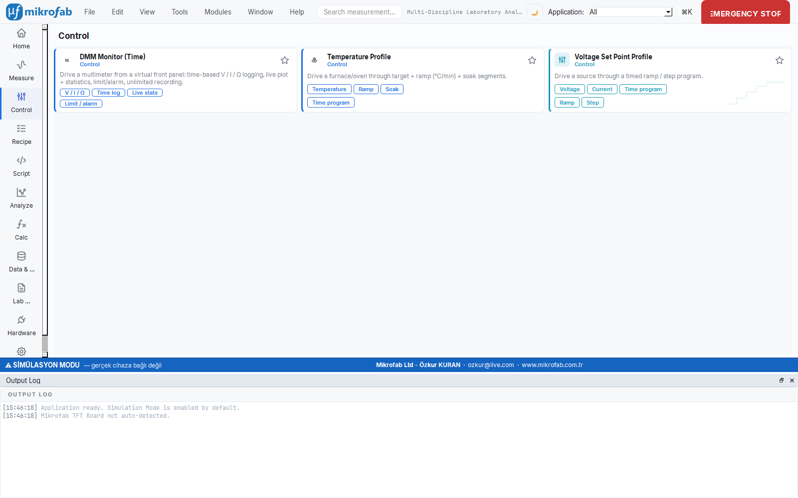
A recipe is the way to run several measurements in a predefined order, like a cooking recipe, without standing over them. You set it up once; the software carries out the steps in order on its own, repeating them across many devices if you wish.
- Why it is done: to relieve you of starting repetitive or long measurement sequences one by one by hand.
- What it teaches / measures: it produces a standard flow (e.g. before/after stress, or measure → analyze → report) consistently and reproducibly.
- Where it is used: stability/overnight tests, multi-device wafer sweeps and end-to-end automated reporting.
The recipe covers two distinct tools for running several measurements as an automated sequence: the classic "stress recipe" (stability/overnight tests) and the new cross-domain "pipeline" (Measure → Analyze → Calc → Report).
4.1 Classic Recipe — Transfer-Before / Bias / Transfer-After
The classic recipe is the standard way to measure how much a TFT degrades over time: it first takes a transfer curve, then subjects the device to voltage stress for a while, and finally takes a new transfer curve to show how much the threshold voltage has shifted (ΔVth). Like wearing out a tire on a long road and comparing before and after.
- Why it is done: to measure the device's stability/lifetime and the threshold shift under bias.
- What it teaches / measures: the post-stress threshold shift (ΔVth) and hysteresis; that is, the device's reliability.
- Where it is used: stability tests that run for hours/overnight and reliability qualification.
The classic recipe is the standard flow for measuring TFT stability: take a transfer curve before stress, then apply bias-stress for a while, then take the post-stress transfer curve and observe the threshold shift (ΔVth). The recipe panel (RecipePanel) offers these controls:
- Browsing the TFT list: Checkboxes are created from the
tft_mappingkeys in the configuration; the recipe is repeated in turn for each TFT you select. This lets you sweep many devices on a wafer with a single start in a relay/switch-matrix setup. - Sequence steps: "Transfer-Before", "Bias Stress", "Transfer-After" and "Dual axis" (dual-axis plot) checkboxes. You can turn off any step (e.g. stress only).
- Role automation (relay): Before the flow starts for each TFT, the switch matrix is routed to that device's drain/gate channels; in modes other than DIODE, if
relay_enabledis set, the relay configuration is applied automatically. The operator does not need to change cables.
The flow (RecipeMeasurementRunner) carries out the following for each selected TFT:
for tft in selected_tfts:
    [Transfer-Before]  → TransferSweep (Dual direction, log scale)
    [Bias Stress]      → BiasStress (Voltage Bias, duration + sampling interval)
    [Transfer-After]   → TransferSweep (Dual direction, log scale)
The transfer sub-sweeps are taken bidirectionally (Dual) so that hysteresis and ΔVth can be extracted; each step is tagged with its own user_comment (recipe transfer before / recipe bias stress / recipe transfer after).
Recipe parameters
| Parameter | Unit | Description | Default |
|---|---|---|---|
selected_tfts | — | List of TFTs over which the recipe is repeated | ["TFT 1"] |
run_transfer_before | — | Take transfer before stress | True |
run_bias_stress | — | Apply bias-stress | True |
run_transfer_after | — | Take transfer after stress | True |
transfer_vds | V | Fixed Vds of the transfer sub-sweep | 1.0 |
transfer_vgs_start | V | Transfer Vgs start | -10.0 |
transfer_vgs_stop | V | Transfer Vgs stop | 10.0 |
transfer_vgs_step | V | Transfer Vgs step | 0.5 |
stress_vds | V | Vds during stress | 1.0 |
stress_vgs | V | Vgs during stress | 10.0 |
bias_duration_s | s | Total stress duration | 3600.0 |
bias_sample_interval_s | s | Stress sampling interval | 10.0 |
bias_duration_s = 28800 for 8 hours) or by combining it with --repeat / --interval in headless mode. Because each point is written to disk immediately during long measurements (*_partial.csv), the data captured so far is preserved even if power is lost (see §5.4).4.2 New Recipe Pipeline (Measure → Analyze → Calc → Report)
The pipeline is an end-to-end chain that, within a single recipe, not only takes the measurement but also automatically analyzes, computes and turns the result into a finished HTML report, like an assembly line. The steps are connected by name; each step takes the output of the previous one as input.
- Why it is done: to run the entire path from raw data to finished report without human intervention, reproducibly.
- What it teaches / measures: it delivers the measurement + extracted metrics + report as a single, auditable output chain.
- Where it is used: standardizing routine characterization and automated reporting (e.g. TFT On/Off, PV Jsc/Voc/FF/PCE).
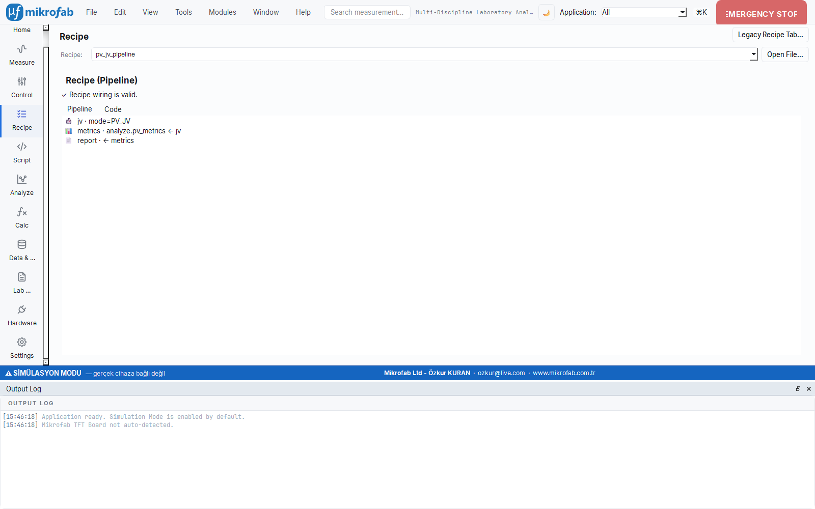
The main view of the recipe workspace is the modern pipeline, which treats data as the single source of truth. A recipe is JSON made of sequentially connected, named, typed steps, and the human-readable Python view is generated from it (one-way; editing the recipe edits the JSON). The step types:
Step (kind) | Function | Core fields |
|---|---|---|
measure | Runs a measurement mode | name, mode, tft_id, params, required_capabilities |
analyze | Applies an analysis module to a previous measurement / file | name, module, source or path, params |
calc | Runs a calculation module with explicit inputs | name, module, inputs |
report | Generates an HTML report from upstream steps | name, title, sources |
Steps are connected by name: every producing step has a unique name; downstream steps reference the upstream output by that name (source / sources). During loading, validate_wiring checks the wiring (unique name, an analysis bound to exactly one source, report sources from previous steps). The recipe page presents the bundled example recipes (examples/recipes/*.json) in a dropdown, you can load your own recipe with "Open file…", and the "Legacy Recipe Tab" button opens the classic recipe runner.
The two bundled examples:
tft_transfer_pipeline.json— measure TRANSFER →analyze.tft_on_off(On/Off + Vth) → HTML report.pv_jv_pipeline.json— measure PV_JV →analyze.pv_metrics(Jsc / Voc / FF / PCE) → report.
report step produces an integrity-sealed HTML report from the outputs of the upstream steps.calc step carries only a module identifier + inputs). This provides a safe and auditable automation chain.5. Headless Mode
Headless mode means running the software from the command line without opening any window — like driving an instrument by remote control. You provide a job file, and the software performs the measurements on its own; if you wish, you control it from other programs via a REST API.
- Why it is done: to set up scheduled and repetitive automation (especially overnight runs) without waiting at the screen.
- What it teaches / measures: it produces the same measurements, but triggered by script/remote rather than by hand and repeated in loops.
- Where it is used: overnight stability runs, server/automation pipelines and remote control.
Headless mode lets you run measurement/automation without opening the GUI: it is designed for overnight recipes, scheduled repeated measurements and remote control. The entry point is the --headless flag of main.py.
python main.py --headless --job examples\job_example.json
python main.py --headless --job recipe.json --output C:\olcumler --repeat 3 --interval 7200
python main.py --headless --serve 8765        # REST API server only
5.1 Command-line flags
| Flag | Argument | Description | Default |
|---|---|---|---|
--headless | — | Run without the GUI | off |
--job | FILE | Job JSON file to run | — |
--output | FOLDER | Output folder (overrides the one in the job) | job / measurements |
--mock | — | Use the mock (hardware-free) driver | per job / True |
--real | — | Use the real device driver | — |
--repeat | N | Total number of cycles (scheduling) | job / 1 |
--interval | SECONDS | Wait between cycles | job / 0 |
--serve | [PORT] | Start the local REST API | port 8765 |
--host | ADDRESS | REST API host | 127.0.0.1 |
--smu-model | MODEL | Real device SMU model key (e.g. 2614B) | — |
--smu-resource | VISA | VISA resource (e.g. GPIB0::26::INSTR) | — |
--formats | LIST | Export formats (csv,txt,xlsx,hdf5) | csv,txt,xlsx |
--sequence | FILE | Run a general Sequence Builder JSON headless | — |
--mock is the default. To connect to a real device you must pass --real (or "mock": false in the job) and provide the SMU model/resource information. The real-hardware path also preserves timeout + safe-state + mock-equivalent behavior (device-communication safety rules).5.2 Job JSON schema
A job JSON file defines one or more measurements to run without the GUI.
| Key | Type | Description | Default |
|---|---|---|---|
mock | bool | Hardware-free simulation | true |
output_directory | str | Output folder | "measurements" |
relay_enabled | bool | Switch-matrix automation (applied except for DIODE) | false |
schedule.interval_s | number | Seconds between cycles | 0 |
schedule.repeat | number | Total number of cycles | 1 |
measurements[] | array | Measurement definitions (at least 1, required) | — |
measurements[].mode | str | Measurement mode (converted to uppercase) | — |
measurements[].tft_id | str | Sample/device identifier | "TFT 1" |
measurements[].user_comment | str | User comment | "" |
measurements[].params | object | Mode-specific parameters (unknown fields are ignored) | {} |
smu | object | Real-hardware SMU connection (model, resource) | {} |
relay | object | Real-hardware relay connection | {} |
Valid mode values: IV, TRANSFER, DIODE, BIAS_STRESS, HW_SWEEP, HW_TFT_SWEEP, PULSED_IV, PV_JV, PV_PULSED_JV, PV_DARK_JV, PV_HYST, PV_MPPT, PV_BIAS_DELTA, PV_SUNS_VOC, PV_INTENSITY, PV_SOAK, PV_DEGRAD, PV_THERMAL, PV_CV, PV_CI, RECIPE. An unknown mode raises an error; for each mode only the parameter fields belonging to that dataclass are accepted, and the rest are silently dropped.
Example (examples/job_example.json): every two hours, three cycles; one TRANSFER + one IV.
{
  "mock": true,
  "output_directory": "measurements",
  "relay_enabled": false,
  "schedule": { "interval_s": 7200, "repeat": 3 },
  "measurements": [
    {
      "mode": "TRANSFER",
      "tft_id": "TFT 1",
      "user_comment": "Overnight stability test",
      "params": {
        "fixed_vds": 1.0, "vgs_start": -5.0, "vgs_stop": 5.0, "vgs_step": 0.25,
        "mobility_method": "Saturation", "w_um": 100.0, "l_um": 10.0, "cox_nf_cm2": 34.5
      }
    },
    {
      "mode": "IV",
      "tft_id": "TFT 2",
      "params": { "vds_start": 0.0, "vds_stop": 5.0, "vds_step": 0.5,
                  "vgs_start": 0.0, "vgs_stop": 5.0, "vgs_step": 1.0 }
    }
  ]
}
5.3 Repeat / interval (overnight tests)
With --repeat N --interval S (or schedule in the job), the measurements in the job are repeated for N cycles, waiting S seconds between cycles. At the start of each cycle === Cycle k/N === is logged, and for each measurement the start and result (point count + files written, or an error) are logged. The wait is done with an interruptible sleep; you can stop cleanly with Ctrl+C (the safe state is triggered). The return value is the number of failed measurements (0 = all succeeded); the process exit code is set to 0/1 accordingly.

5.4 Outputs
Each run is written to a unique subfolder under your output folder: YYYY-MM-DD-<Day>-<Kind>-<HHMMSS> (e.g. 2026-06-12-Wed-PV-103045). <Kind> is the abbreviation of the measurement family (TFT / Thin / PV / Gen). The trailing hour-minute-second makes each run unique, so that no multi-machine conflict copies are created in synced folders such as OneDrive.
The files a measurement produces:
| File | Content |
|---|---|
<name>.csv | Raw points (comma-separated) |
<name>.txt | Raw points (tab-separated) |
<name>.xlsx | Excel (measurement sheet + a separate "Summary" sheet) |
<name>_metadata.json | Full data sheet (device identity, parameters, summary, point count, early-stopped) |
<name>_report.json | Canonical integrity-sealed report (checksum included) |
<name>_report.csv | Locale-independent report CSV |
<name>.h5 | (optional) Sealed HDF5 binary output |
<name>_partial.csv | Crash-resilient file updated at every point during the measurement (deleted on successful completion) |
metadata.json are always preserved. If openpyxl is not installed, the software still produces a minimal XLSX with the standard library.6. Local REST API
The REST API lets you manage the running measurement controller with HTTP commands like a remote control: start/stop a measurement, read the status and live data. This way another program, script or browser can drive the measurement from the outside.
- Why it is done: to expose the measurement to other software/automation or to a remote machine.
- What it teaches / measures: it returns the instantaneous status (running or not, how many points, last error) and the live data captured so far.
- Where it is used: laboratory automation integration, remote monitoring and custom control panels (only on a trusted/local network).
The REST API started with --serve lets you control/monitor a running controller (HeadlessController) over HTTP. Only the Python standard library is used (no extra dependency), and by default it binds to localhost only (127.0.0.1).
6.1 Endpoints
| Method | Path | Function | Response |
|---|---|---|---|
| GET | /health | Health + version | {"ok": true, "version": "…"} |
| GET | /status | Controller status | the status object below |
| GET | /data/live (or /measurement/data/live) | All points captured so far | {"points": [ … ]} |
| POST | /measurement/start | Start a measurement | 200 started / 409 busy / 400 invalid parameter |
| POST | /measurement/stop | Stop the measurement safely | {"stopped": true} |
Unknown paths return 404. The /status object: running, mode, point_count, last_error, last_paths, last_point for the last point (step_index, vds, vgs, ids, igs, elapsed_s) and, if present, summary.
6.2 Request examples
The measurement start body: mode (required), tft_id (default "TFT 1"), params (mode-specific), relay_enabled (ignored for DIODE).
# Health check
curl http://127.0.0.1:8765/health

# Start a transfer measurement
curl -X POST http://127.0.0.1:8765/measurement/start \
     -H "Content-Type: application/json" \
     -d '{"mode":"TRANSFER","tft_id":"TFT 3",
          "params":{"fixed_vds":1.0,"vgs_start":-5,"vgs_stop":5,"vgs_step":0.25}}'

# Fetch live data
curl http://127.0.0.1:8765/data/live

# Stop
curl -X POST http://127.0.0.1:8765/measurement/stop
If a measurement is already running, a start call returns 409 ("Measurement already in progress"); if the parameters are invalid, 400 and an error message are returned.
--host but always keep it behind a trusted network / VPN / reverse proxy. Do not expose it directly to the open network.7. Python Script / Console
The Script workspace lets you drive the measurement engine with your own sentences — Python commands — instead of ready-made buttons. You type in a terminal or write and run a small program, then plot and analyze the results in the same place.
- Why it is done: to flexibly build custom measurement/analysis flows that the ready-made panels do not cover.
- What it teaches / measures: it exposes measurement, SMU control, analysis and plotting as a fully programmable API.
- Where it is used: R&D, custom experiment design and expert users who automate repetitive work.
The Script workspace drives the software's measurement core through a Python scripting API. It opens from the "Script" card on the left rail; it offers full programmability for experts and R&D. It runs against the Qt-independent app.scripting core.
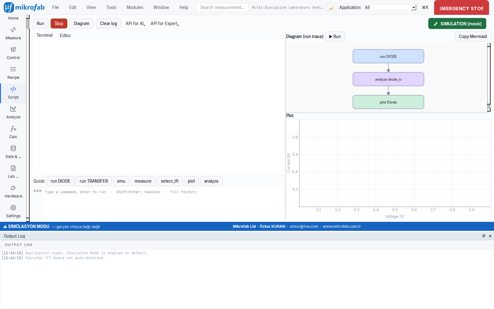
7.1 Layout: Terminal + Editor, Plot + Diagram
- Terminal (primary surface): Like a real terminal, it echoes the
>>>input and prints the response inline. Multi-line input: Enter runs, Shift+Enter adds a new line, ↑/↓ navigates history, and multi-line paste works. Each submission runs on a worker thread against a persistent session, sowait(...)does not freeze the interface and variables are preserved between commands. - Editor: A full 15–20 line program. The Run / Diagram buttons on the toolbar act on the editor code; output streams to the same Terminal.
- Plot:
plot()calls overlay I–V curves (they stack within a run). - Diagram: Draws the recorded run trace as a flowchart; with Copy Mermaid it exports it as portable text (drawn automatically in the background with debounce as you type in the editor).
7.2 API functions (quick-access examples)
The quick-action buttons below the terminal place frequently used calls into the input:
| Button | Example call |
|---|---|
| run DIODE | run("DIODE", voltage_start=0.0, voltage_stop=2.0, voltage_step=0.05) |
| run TRANSFER | run("TRANSFER", fixed_vds=0.1, vgs_start=-10, vgs_stop=10, vgs_step=0.2) |
| smu | smu("drain").set_voltage(0.1, compliance_a=1e-3) |
| measure | measure("drain") |
| select_tft | select_tft(1) |
| plot | plot(res, title="IV") |
| analyze | analyze(res, "diode_iv") |
A typical script:
res = run("DIODE", voltage_start=0.0, voltage_stop=2.0, voltage_step=0.05)
extra = analyze(res, "diode_iv")
log(f"n={extra.ideality_factor}  I0={extra.saturation_current}")
plot(res, title="Diode")
7.3 Simulation / Live badge and safe state
The large colored badge on the toolbar shows the operating mode: green = Simulation (Mock), red = Live (real device). Scripts run in simulation by default (safe to write, hardware-free). You switch to Live by clicking the badge. When the mode is changed, "Stop" is pressed, you leave the workspace, or the session is reset while outputs are on, the software enters the safe state (output OFF + relay OFF) — a manually held bias never outlives the page.
7.4 API export for AI and experts
There is no embedded artificial intelligence or network connection inside it. Instead: API for AI copies a single-page API definition to the clipboard/Markdown (which you give to your own AI assistant); API for Expert downloads a multi-file package (type stub .pyi + cheat sheet + examples ZIP). This way you can write the script with an external LLM and paste it here.
8. Presets, Configuration, Favorites and User Modes
8.1 Configuration (ConfigManager)
Settings are two-layered: the bundled default_config.json and the user user_config.json; the latter is deep-merged over the former (_deep_update). Some keys are deliberately not overridable by the user and always come from the default:
- Safety limits (
safety_limits): Per customer request, the software does not impose artificial limits; the limit is always read fromdefault_config.json. This way a low value in an olduser_config.json(e.g. 60 V) does not get stuck, and the higher value you enter is not rejected at the start of the measurement. - Feature flags (
ui_lcr_pv,ui_rps,ui_dmm…) are also pinned: so that a blanketsave()does not write back a stalefalsevalue and silently override a new default. To turn these off, environment variables (MIKROFAB_LCR_PV=0,MIKROFAB_RPS=0,MIKROFAB_DMM=0) are used.
8.2 Preset manager (PresetManager)
A preset is saving your frequently used measurement settings under a name and recalling them with a single click — like the saved numbers on your phone. Because different materials/technologies want very different voltage ranges, you keep a separate preset for each.
- Why it is done: to avoid re-entering dozens of parameters by hand for every measurement and to avoid mistakes.
- What it teaches / measures: it stores a panel's entire parameter state as a named, reusable set.
- Where it is used: quickly switching between different technologies such as a-Si / IGZO / organic and standard measurement setups.
It saves/loads named parameter sets to disk for each measurement panel. Different TFT technologies (a-Si, IGZO, organic) want very different parameter ranges; presets enable quick switching between these sets. The directory structure:
<root>/presets/<panel_key>/<preset_name>.json| Operation | Behavior |
|---|---|
list(panel) | Returns the panel's preset names alphabetically |
save(panel, name, state) | Saves the state dictionary as JSON (name file-safe, ≤80 characters) |
load(panel, name) | Reads a preset and returns the state dictionary |
delete(panel, name) | Deletes the preset (silently passes if it does not exist) |
8.3 Favorites / recently used and user modes
- View profiles (Data panel): The named column/sort/filter layouts described in §2.3 act in practice as "favorite views"; you bring back frequently used analysis angles with a single click. The active profile is stored in the configuration (
db_active_profile) and restored on startup. - Recently used recipes: The recipe page automatically loads the first of the bundled recipes on startup and preserves the last selection even across a language change.
- User modes: The complexity of the interface scales to your role via the User Mode setting (Operator / Expert / Developer); advanced tools such as Script and headless typically come to the fore in Expert / Developer modes (for details see the Introduction chapter §11).
9. Backup and Integrity
These tools protect the safety and soundness of your data like an insurance policy: they take a consistent copy of the database, test whether it is corrupted, and keep a who/when/why record of every change.
- Why it is done: to protect against data loss, corruption and the uncertainty of "who changed this record?".
- What it teaches / measures: it ensures the consistency of the backup, database integrity and a full audit trail.
- Where it is used: routine backup and laboratories that require accredited (ISO 17025 / 21 CFR Part 11) traceability.
Each database (measurement + Lab Notebook) offers its own consistent backup and integrity check:
| Operation | Description |
|---|---|
backup(path=None) | Takes a consistent copy with the SQLite online backup API; if no path is given, db_backups/…<time>.db |
| Pre-migration backup | Automatic before a version upgrade (pre_migration_vN) |
| Pre-hard-delete backup | Automatic before hard_delete (pre_hard_delete) |
check_integrity() | PRAGMA integrity_check; True if the database is sound |
audit_trail(entity_id=None) | Lists the audit records (all of them or for a single record) |
audit_log), soft-delete and pre-migration backup provide the foundation of that compliance out of the box: every create/update/delete/restore stores who (actor) and why (reason), along with a full snapshot before the change (before_json).