Academy / Education

Learn characterization: how do parameters emerge from a graph?

A device's threshold voltage, its mobility, or a solar cell's efficiency don't appear out of thin air; they are all read from a measured curve through a handful of fundamental graphical operations. This page explains those operations — taking a slope, drawing a tangent and extending it (extrapolation), together with log / √ / log-log transforms — in a tutorial style, through annotated diagrams.

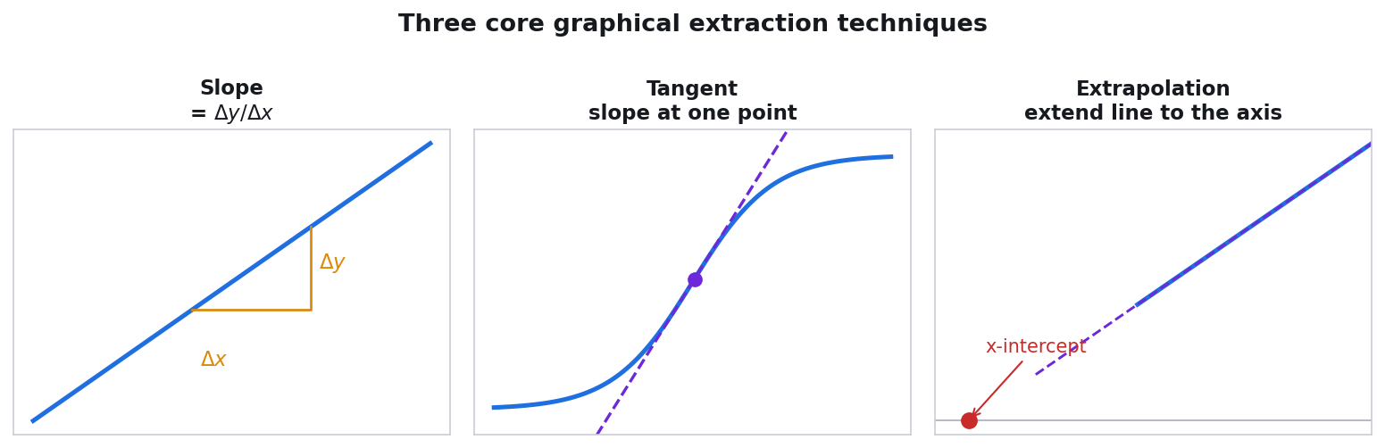
The three fundamental graphical techniques of characterization: taking the slope of a curve, drawing a tangent at the steepest point, and reading an intercept by extending the tangent/fit line to an axis — Three core techniques together: taking a slope (yields a rate), drawing a tangent (builds a linear model) and extending/extrapolating (reveals a hidden intercept). Every method that looks complicated is just a repetition of these ideas.

Modern characterization may look complex, but underneath it lies a few recurring ideas. Taking the slope of a curve gives a rate/ratio (transconductance g_m, subthreshold swing SS, ideality factor); drawing a tangent at the steepest point and extending it reveals a hidden intercept (threshold voltage V_th, built-in voltage V_bi, saturation current I₀); and moving the curve onto a log, square-root or log-log axis turns a curved relationship into a straight line, so that slope and intercept can be read with confidence.

📈

Taking a slope

The local slope (derivative) of a curve gives a rate: g_m = dI_d/dV_gs, the subthreshold swing SS, or the ideality factor from the slope of ln(I)–V. The numerical derivative is computed with the central difference, and one-sided at the endpoints.

📐

Drawing a tangent

Drawing a tangent at the steepest (most informative) point of the curve is the first step toward building a linear model; the equation of that tangent is then extended onto an axis in the next step.

↘️

Extrapolation (extending)

Extending the tangent or fit line to an axis and reading its intercept yields a hidden quantity: V_th (x-intercept), I₀ (y-intercept), built-in voltage V_bi.

🔁

Transformation

A log, √ or log-log axis is used to straighten a curved relationship: ln(I)–V for a diode, √I_d–V_gs in saturation, log–log power-current for a photodetector.

37

measurement modes

37

analysis modules

8

Calc compute engines

9

techniques covered in this lesson

ℹ️

This page is a tutorial overview. For the full derivation of each formula, its validity limits, constants (CODATA 2019) and standard references, see the Calculation Workshop and Physics Reference section of the Manual.

Transistor (TFT / FET)

Threshold, slope and mobility from the transfer curve

A single transfer curve (I_d–V_gs, at fixed V_ds) yields the threshold voltage, the subthreshold swing and the mobility all at once — as long as you apply the right graphical operation to each.

Threshold voltage V_th — tangent extrapolation

The classic example of the “draw a tangent + extend it” combination. A tangent is drawn to the curve at the point of maximum transconductance, and this tangent is extended until the current reaches zero; where the tangent crosses the x-axis gives the threshold voltage.

What we measure: The gate voltage at which the channel turns on.
Which graph: I_d–V_gs in the linear region.
Which operation: Tangent at the g_m,max point → extend to the x-axis.
Result: V_th = V_gs* − I_d*/g_m,max

The √I_d–V_gs plot is also linear in saturation; the x-intercept of that line likewise gives V_th (the √I_d method). The Ghibaudo Y-function (Y = I_d/√g_m) is a third route that is robust to series resistance. Standards: IEC 60747-7, IEEE 1620.

TFT / transfer measurements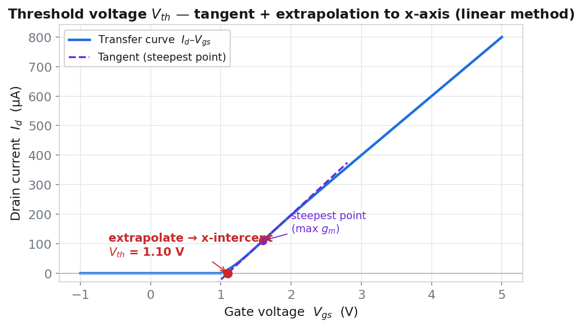

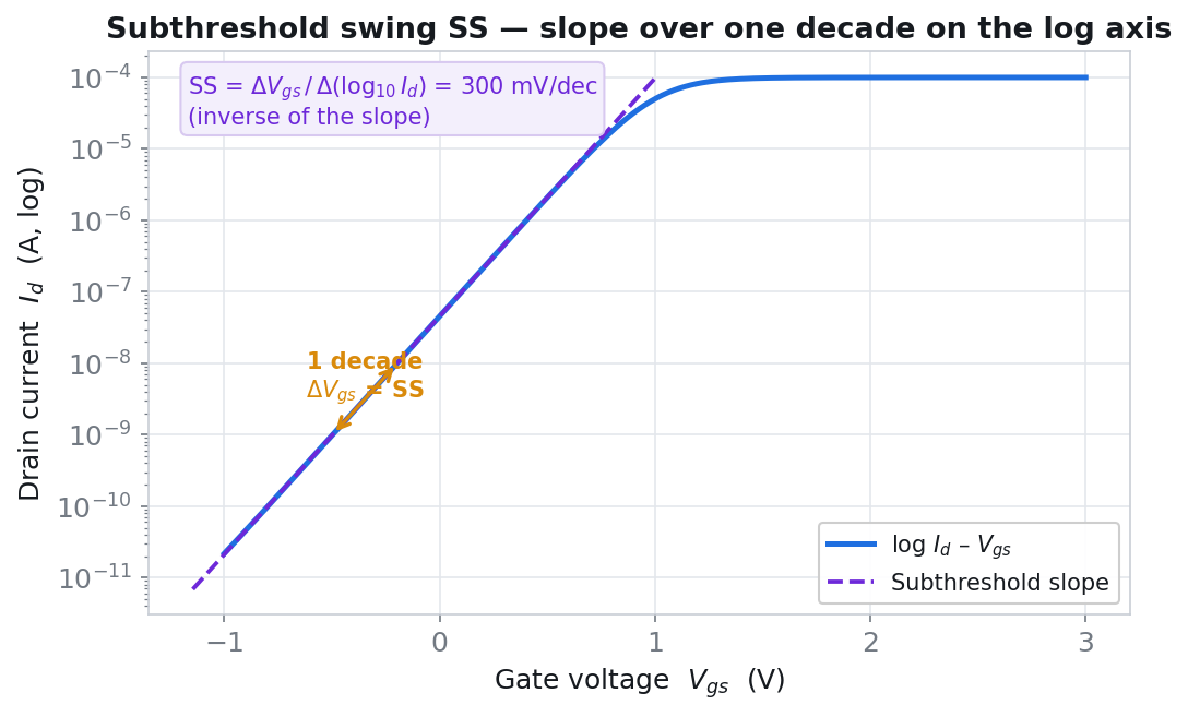
Reading the threshold voltage V_th by extending the tangent drawn at the maximum-transconductance point of the transfer curve to where the current axis crosses zero — The tangent drawn at the g_m,max point is extended to the x-axis; the intercept is V_th.

Subthreshold swing SS

Here it is enough to move a curve onto a log axis and take its slope. It measures how much gate voltage is needed to increase the current tenfold; it tells you how sharp the switching is.

What we measure: The V_gs needed to raise the current by one decade (×10).
Which graph: log₁₀|I_d|–V_gs (semi-logarithmic).
Which operation: Take the slope at the steepest part of the subthreshold region, then invert it.
Result: SS = dV_gs / d(log10 I_d) [mV/dec]

At 300 K the thermal limit is ~59.53 mV/dec; values below it (without a ferroelectric gate) are physically impossible — the software still reports the value but leaves a warning rather than silently correcting it. The interface trap density also follows from SS: Dit = (Cox/q)·(SS/SS_ideal − 1).

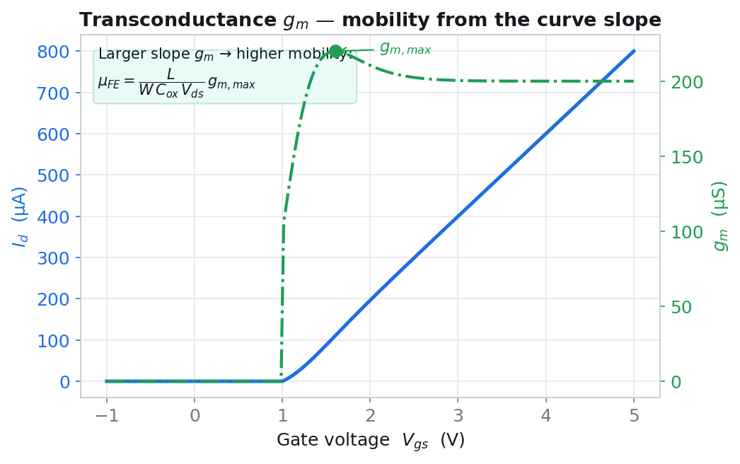
Computing the subthreshold swing SS from the steepest linear portion of the subthreshold region of a semi-logarithmic transfer curve — The steepest slope of the subthreshold region is taken on a semi-log axis; SS = 1/slope.

Field-effect mobility µ_FE

Mobility comes from the peak value of the slope (g_m) of the transfer curve. It measures how easily carriers drift through the channel.

What we measure: Ease of carrier drift (cm²/Vs).
Which graph: g_m = dI_d/dV_gs (derivative of the transfer curve).
Which operation: Take the peak of g_m, then scale by the geometry.
Result: µ_FE = g_m,max·L / (W·Cox·|Vds|)

The saturation mobility µ_sat comes from the slope (m) of the √I_d–V_gs line: µ_sat = m²·2L/(W·Cox). Because W/L is taken as dimensionless, the result comes out directly in cm²/Vs; there is no factor of 10⁴.

Field-effect mobility computed from the peak of the transconductance g_m curve, which is the derivative of the transfer curve — The peak of the g_m curve (g_m,max), scaled by the geometry, gives µ_FE.

Diode and semiconductor interface

Reading hidden parameters with the logarithm and 1/C²

Exponential and quadratic relationships cannot be read directly; but with the right transform they turn into a straight line. The slope and intercept then give the diode quality and the interface doping.

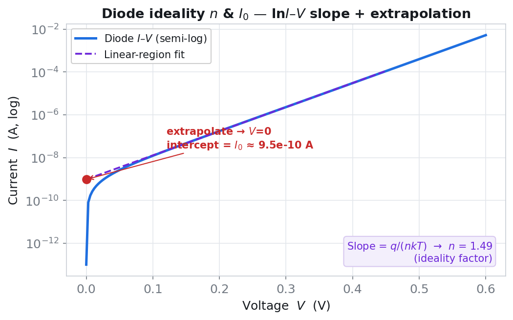
Diode ideality factor n

Moving the exponential I–V onto a logarithm turns it into a straight line; the slope gives the ideality, the intercept gives the saturation current. n = 1 indicates ideal Shockley behavior, while a large n indicates recombination/series-resistance effects.

What we measure: Deviation from ideal diode behavior (n) and the saturation current I₀.
Which graph: ln(I)–V (forward bias, semi-logarithmic).
Which operation: Take the slope over the linear mid-region; extend the line to V=0 and read the intercept.
Result: n = q/(kB·T·slope), I0 = exp(intercept)

For series resistance, the Cheung method uses the dV/d(ln I) plot; the Schottky barrier Φ_B is found from I₀ via thermionic emission. In a typical example n ≈ 1.5 is obtained. Standards: Schroder, Cheung.

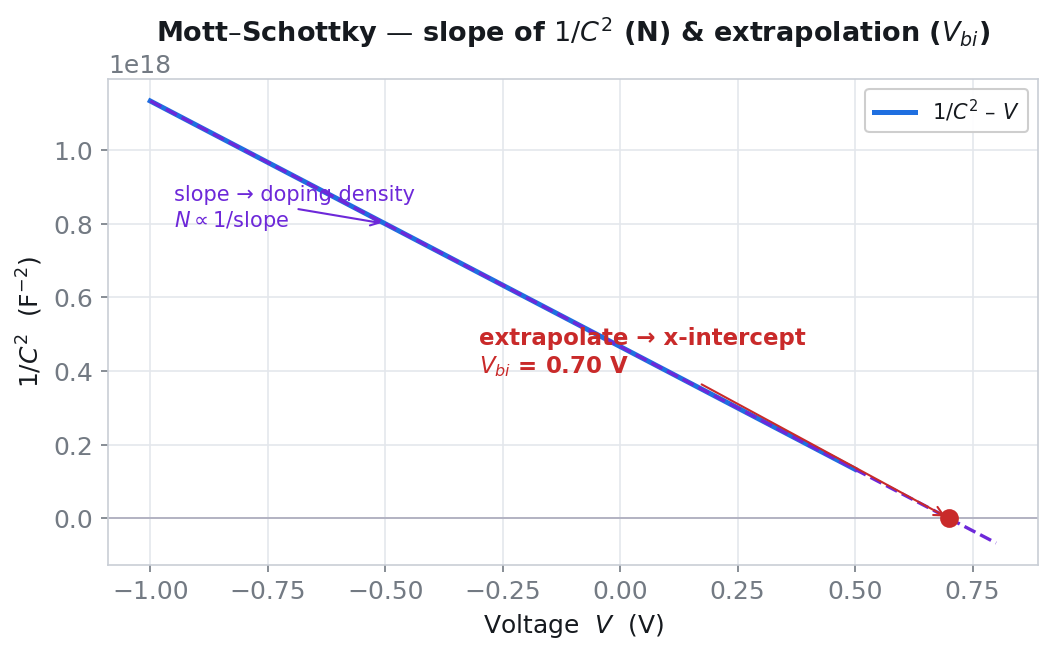
Extracting the ideality factor from the slope of the linear region and the saturation current I0 from the y-intercept on a plot of the logarithm of the diode forward current versus voltage — The slope of the ln(I)–V line gives n, and extending it to the y-intercept gives I₀.

Mott-Schottky — doping and built-in voltage

Taking the inverse square of the capacitance linearizes the depletion physics. The slope of the line fitted to the linear region gives the effective doping, and extending it to the x-axis gives the built-in voltage.

What we measure: The effective doping density N_eff and the built-in voltage V_bi.
Which graph: 1/C²–V (derived from a C–V sweep).
Which operation: Fit the linear region; N_eff from the slope, V_bi from extending to the x-intercept.
Result: N_eff = −2/(q·ε_r·ε0·A²·m), V_bi = −b/m, W_d = ε_r·ε0·A/C

The uncertainty comes directly from the fit covariance: u(N)/N = u(m)/|m|. Standard: Sze, Physics of Semiconductor Devices.

Extracting the effective doping from the slope of the linear fit and the built-in voltage V_bi from the x-intercept on a Mott-Schottky plot of the inverse square of capacitance versus voltage — The slope of the 1/C²–V line gives N_eff, and the x-intercept gives V_bi.

Photovoltaics and photodetectors

Efficiency from a curve's area, speed from time, responsivity from a ratio

Optoelectronic characterization rests on the same three ideas: finding a maximum on a curve, reading the levels along a time axis, and taking the ratio of two quantities.

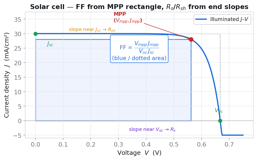
Solar cell fill factor FF

FF measures the “rectangularity” of the illuminated J–V curve — that is, the balance between series and shunt resistance. You find the point on the curve where the power (J·V) is greatest and take its ratio to the corner values.

What we measure: Curve quality (FF) and power conversion efficiency (PCE).
Which graph: Illuminated J–V curve (power quadrant).
Which operation: Find the maximum power point (J_mp·V_mp largest); take its ratio to the corner values.
Result: FF = (Jmp·Vmp)/(Jsc·Voc), PCE = (Jmp·Vmp)/Pin·100

Under standard conditions (AM1.5G, 100 mW/cm², 25 °C) a practical shortcut holds: PCE[%] = Jsc·Voc·FF. In a physical cell 0 < FF < 1; FF > 1 signals a sign/turning-point error. Standard: IEC 60904-1.

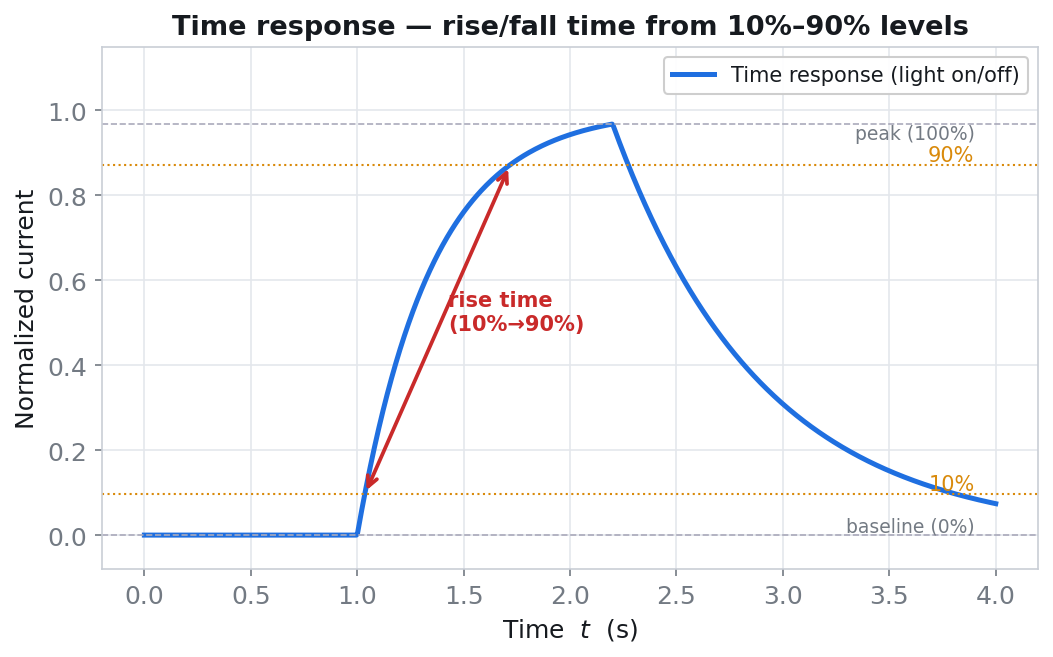
Illustration of the maximum power point and the rectangle that defines the fill factor on a solar cell illuminated J-V curve — The ratio of the maximum power rectangle to the J_sc·V_oc area is the FF.

Photodetector rise time

Here it is not a curve but the time axis that is read. In a light on/off pulse, the speed at which the signal transitions from baseline to peak tells you how quickly the detector responds.

What we measure: The detector's response speed to light and its bandwidth.
Which graph: Current–time (photo-switching pulse).
Which operation: Determine the baseline and peak levels; read the times of the 10% and 90% levels and take their difference.
Result: t_rise = t(90%) − t(10%), BW₋₃dB ≈ 0.35/t_rise

For a single-pole RC system a closed form holds: t_rise = ln(9)·τ = 2.197·τ. Multiple cycles are averaged. Standards: IEEE 181, IEC 60469.

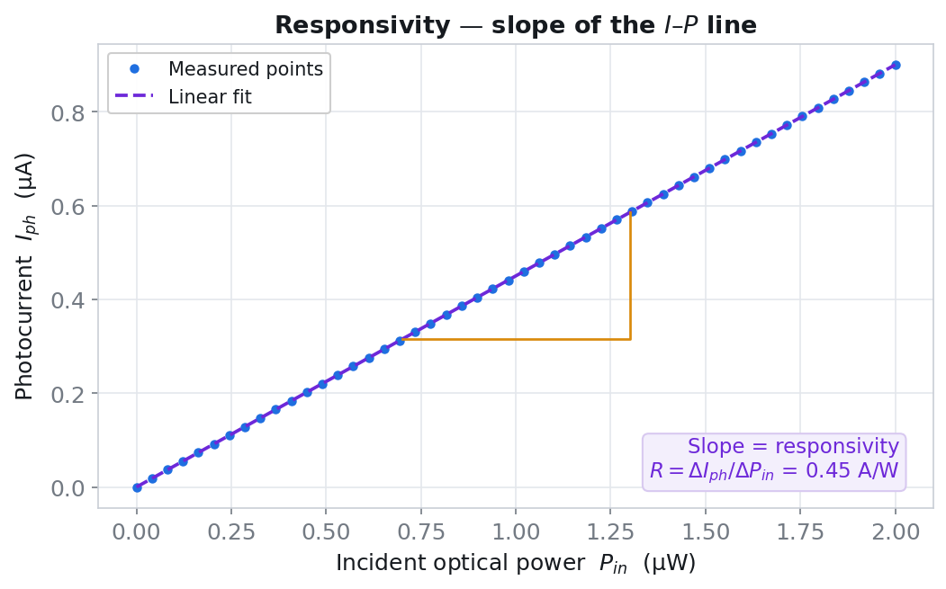
Reading the rise and fall times from the time difference between the 10 percent and 90 percent levels of a photodetector current-time pulse — The time difference between the 10%–90% levels, relative to baseline and peak, is the rise time.

Spectral responsivity

Responsivity is a simple ratio: the net photocurrent divided by the optical power incident on the detector. Plotted against wavelength, it gives the R(λ) curve.

What we measure: The photocurrent produced per unit of optical power.
Which graph: Photocurrent–power (and, where available, responsivity–wavelength).
Which operation: Subtract the dark current; divide by the power incident on the detector.
Result: R = I_photo / P_det [A/W], EQE = R·1239.84/λ

Use the power incident on the detector, not the source power. Example: 0.45 A/W at 850 nm → EQE 65.6%. A log-log power sweep also yields the linear dynamic range (LDR) and the exponent α. Standards: IEC 60904-8/10.

Obtaining the responsivity and the wavelength-dependent R lambda curve from the ratio of net photocurrent to the optical power incident on the detector — The ratio of net photocurrent to detector power gives the responsivity (A/W).

Accuracy and uncertainty

How trustworthy is a slope? Regression and the GUM

Every technique above ultimately comes down to a “slope/intercept reading.” What determines how much you can trust it is the regression that fits that line to the data, and the uncertainty budget.

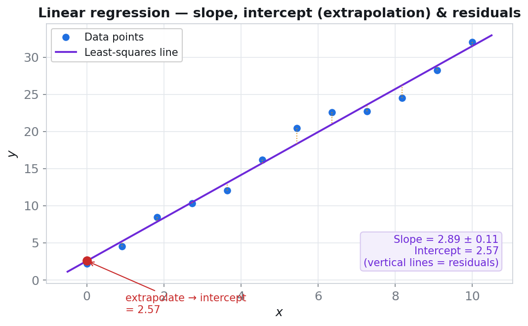
Linear regression and the uncertainty budget

A least-squares (OLS) fit gives not only the slope and intercept but also their uncertainties. The spread of the residuals tells you how well the slope is defined.

What we measure: The slope/intercept and the Type-A uncertainty of each.
Which graph: Any linearized (x, y) scatter.
Which operation: OLS fit; u(m) and R² from the residual variance.
Result: m = Σ(x−x̄)(y−ȳ)/S_xx, u(m) = √(s²/S_xx), U = k·u_c

The software presents every result as value ± U within the GUM (JCGM 100) framework, shows each input's percentage share in the uncertainty budget, and cross-validates non-linear models with Monte Carlo (JCGM 101). Standard: ISO/IEC Guide 98-3.

Applying a linear least-squares fit to data points, showing the uncertainty of the slope and intercept with a confidence band — A least-squares fit yields the slope, intercept and their uncertainties together.

📏

GUM tip. The standard error of a repeated measurement s/√N is Type-A; information from a calibration certificate, a manufacturer's tolerance or resolution is Type-B (e.g. u = a/√3 for a uniform distribution). The combined uncertainty u_c is found by summing in quadrature; the expanded uncertainty is U = k·u_c (k ≈ 2 → ~95% confidence).

Who is it for?

For the classroom, the lab and homework

Designed for everyone from the first-time learner of characterization to the instructor who wants to visualize a lecture; every result is transparent and traceable.

Students

Students and beginners

See where every parameter comes from through annotated diagrams.
Generate and experiment with realistic curves in simulation (mock) mode without any hardware.
Write homework, projects and theses with explicit formulas and standard references.
In the Calculation Workshop, enter values by hand and follow the formula → output → unit step by step.

Academia

Instructors and academics

Ready, consistent visual narratives for lectures and lab sessions.
Every result is traceable: input → formula → output → unit → standard.
Teach measurement accuracy concretely with GUM uncertainty and Monte Carlo.
Record student measurements and procedures with the Lab Notebook (ELN).

Go deeper

Full derivations and measurement practice

For the full mathematics behind every technique summarized in this lesson, and how the curves are acquired on the instrument, take a look at two resources.

Physics reference

Calculation Workshop and Physics Reference

All constants (CODATA 2019), the full formula and validity limits of each quantity, the GUM uncertainty core, and 8 ready compute engines that let you calculate by hand without touching the instrument.

VthSSmobilityidealityMott-SchottkyGUM

Open the physics reference

Measurement practice

Semiconductor / TFT / Diode Measurements

How to acquire transfer, output, I–V, diode/Schottky and pulsed measurements on the instrument — that is, exactly where the curves you take slopes of and draw tangents to in this lesson actually come from.

transferoutput curveI–Vdiodepulsed

Open the measurement guide

Learn characterization by doing

Whether or not you have the hardware: generate realistic curves in simulation mode, apply these techniques yourself, and see the result with explicit formulas plus GUM uncertainty.

Request a demo / trial Open the Manual

Academy — Learn Characterization