CAPABILITIES

What is measured, what is analyzed

Mikrofab Suite brings five major characterization families together in a single application: semiconductor/TFT/diode, photovoltaics, LCR/impedance, resonant acoustic spectroscopy and photodetector. A total of 37 measurement modes generate data from the instrument; 37 analysis modules extract physical metrics from the file you load. Every number comes from a single pure core; measurement, batch processing and the Analysis workspace always return the same result. A value that cannot be computed is never filled with 0 — it is shown as “missing” (—).

37

measurement modes

37

analysis modules

5

characterization families

30+

validated sample data sets

ℹ️

All modules can be tried end to end in simulation (mock) mode without connecting any hardware. Physics-based mock drivers reproduce transistor, diode, solar cell and acoustic resonance behavior realistically, so that every metric is recovered consistently from analysis. On real hardware the same interface and the same analysis flow are used; only the data source changes.

FAMILY 1 · SEMICONDUCTOR / TFT / DIODE

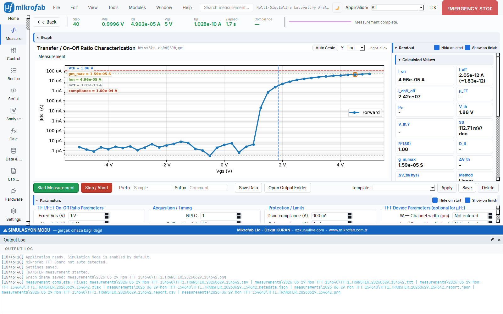
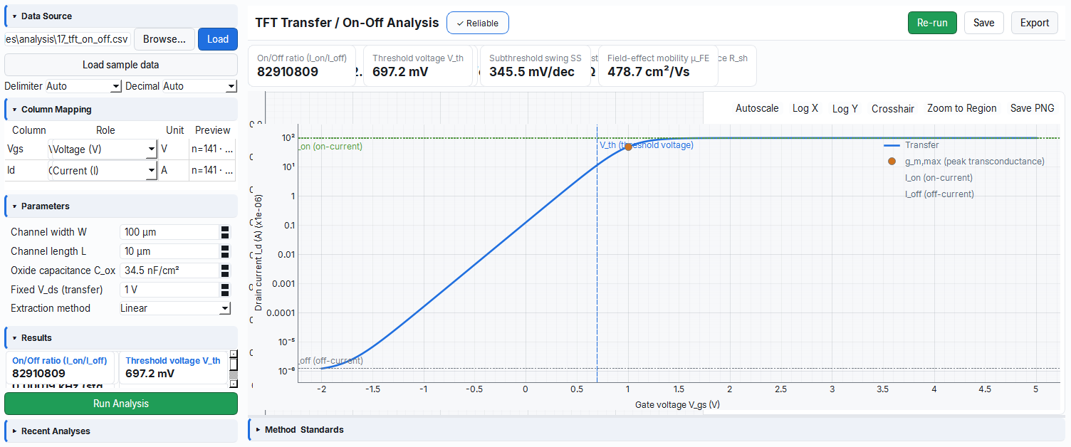
Transistor, diode and resistivity characterization

A broad family ranging from transfer (Id–Vg) and output (Id–Vd) sweeps to pulsed I-V, hardware-fast sweeps, diode/Schottky I-V, reverse recovery, four-point resistivity, van der Pauw/Hall, Kelvin 4-wire and temperature-dependent I-V. Threshold voltage is computed by peak-gm tangent extrapolation (IEC 60747 line), subthreshold swing from the steepest decade window, and mobility with optional geometry (W, L, C_ox).

Transfer / on-off. V_th, SS, µFE/µ_sat, I_on/I_off, g_m,max, Y-function µ0/V_th,Y, interface trap density D_it and hysteresis ΔV_th in dual sweeps.
Output family. R_on, output resistance r_o, channel-length modulation λ, Early voltage V_A, knee voltage and intrinsic gain A_v.
Diode / Schottky. Ideality factor n, saturation current I0, series/shunt resistance R_s/R_sh, rectification ratio RR, Schottky barrier height Φ_B and saturation current density J0.
Reliability & mapping. Bias-stress ΔV_th/MTTF, SET/RESET endurance window and wafer heat-map uniformity.

Read about semiconductor measurements

TFT transfer measurement: drain current versus gate voltage with linear, logarithmic and gm curves plus live Vth/SS/mobility readout

Metric	Symbol	Unit	Method / Basis
Threshold voltage	V_th	V	Peak-gm tangent extrapolation (IEC 60747)
Subthreshold swing	SS	mV/dec	Steepest ~1 decade window; 300 K physical limit ≈ 59.5 mV/dec
Field-effect mobility	µFE / µ_sat	cm²/Vs	From g_m,max or √I_DS slope (with W, L, C_ox)
On/off ratio	I_on/I_off	—	Noise-robust off median; typically ~10⁸
On-resistance	R_on	Ω	Inverse of the low-V_DS linear-region slope
Ideality / saturation current	n · I0	— · A	ln(I)–V fit, shunt-corrected (Shockley)
Schottky barrier	Φ_B	eV	Thermionic emission; Richardson plot in T-IV

FAMILY 2 · PHOTOVOLTAICS / SOLAR CELL

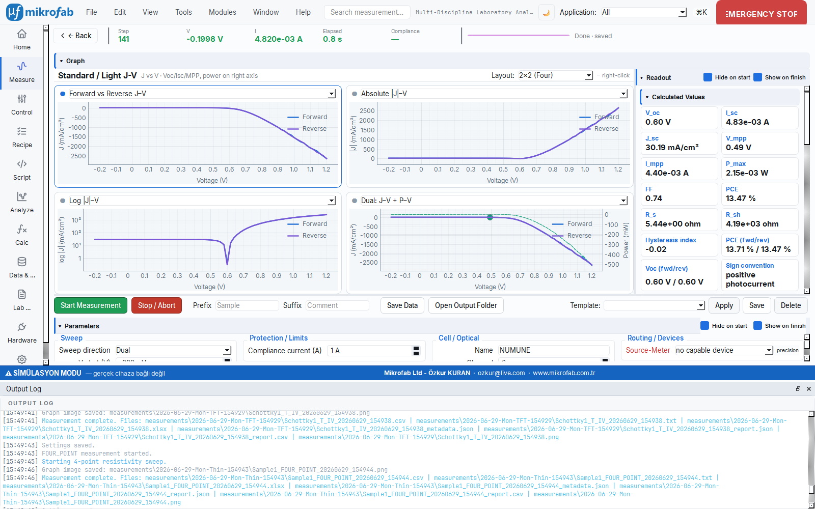
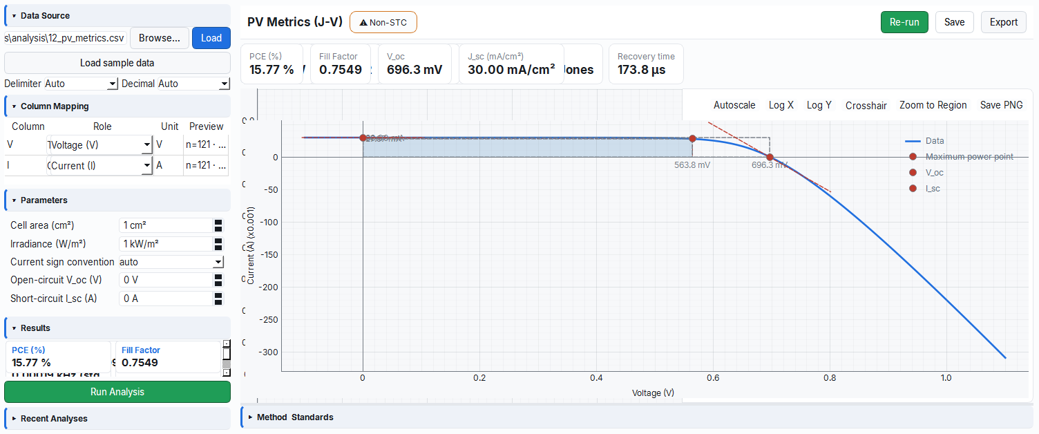
J-V performance and stability metrics

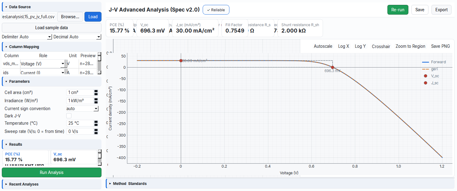
With light/dark/hysteresis/pulsed J-V, Suns-Voc, irradiance sweep, MPP tracking, light soaking, bias-stress, degradation and thermal-stress modules, it characterizes a solar cell, mini-module, perovskite or silicon test structure end to end. All performance metrics are produced from a single core (Spec v2.0); irradiance is entered manually (STC = 1000 W/m², AM1.5G) and active area is mandatory for PCE. The sign convention is detected automatically from the power-quadrant integral.

Core J-V. V_oc, J_sc, V_mpp, P_max, fill factor FF, efficiency PCE and window-fitted series/shunt resistance R_s/R_sh (with reported R²).
Hysteresis. HI = (PCE_rev − PCE_fwd) / PCE_rev and an area-based hysteresis index — an indicator of ion migration/trapping in perovskites.
Stability & aging. Retention (%), T80/T90 lifetime thresholds (ISOS 2020), MPP stability and temperature coefficients dV_oc/dT, dPCE/dT.
Advanced analysis. Suns-Voc ideality factor n, irradiance linearity (J_sc–suns R²) and apparent capacitance / scan-rate dynamics.

Read about photovoltaic measurements

Photovoltaic J-V workspace: forward/reverse J-V, dual J-V plus power curve with marked MPP and live PCE/Voc/Jsc/FF metric cards

PERFORMANCE

V_oc · J_sc · FF · PCE

Open-circuit voltage is taken from the persistent first zero crossing of the current, short-circuit current density from V=0 interpolation, fill factor as P_max/(V_oc·I_sc) and efficiency as P_max/P_in.

IEC 60904-1/3ASTM E948STC

RESISTANCES

R_s · R_sh

Series resistance is extracted by linear fit in the [V_oc, V_oc+0.05 V] window and shunt resistance in the V=0 ± 0.05 V window; if the window is insufficient it falls back to the local slope.

window-fitR² reported

STABILITY

Retention · T80 / T90

From light-soaking and degradation runs, the retained percentage relative to the start and the time to first reach 80%/90% of PCE (linear interpolation, exponential extrapolation if needed).

ISOS 2020PCE(t)

FAMILY 3 · LCR / IMPEDANCE

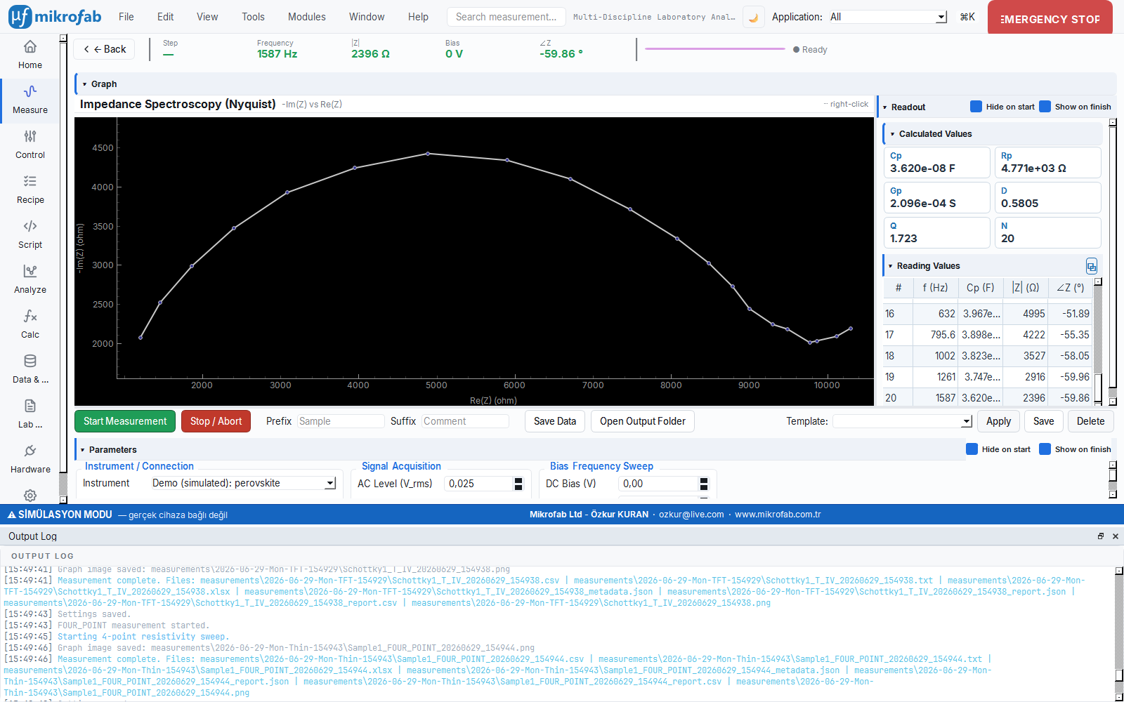
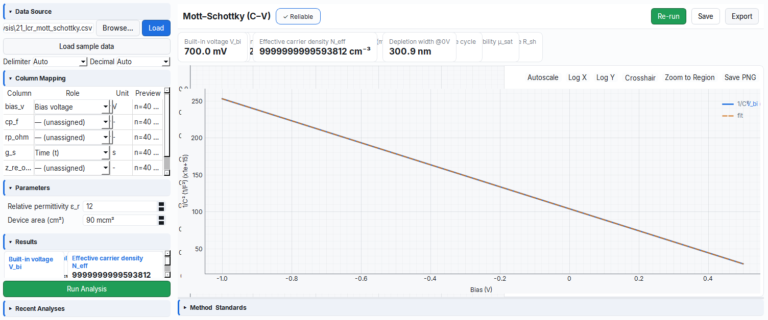
C-V, Mott-Schottky and impedance spectroscopy

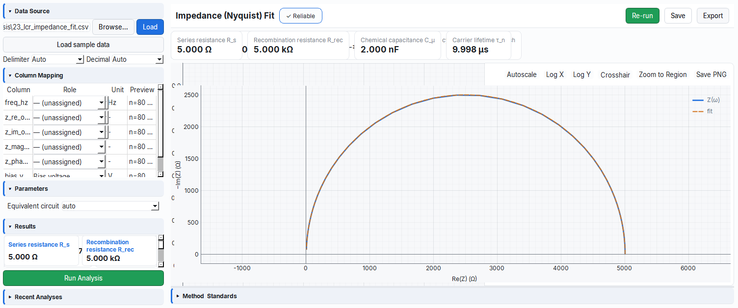
The LCR/impedance workstation gathers four measurement modes in a single form: capacitance–voltage (C-V), capacitance–frequency (C-f), impedance spectroscopy (Z-f, Nyquist) and temperature-resolved admittance (TAS). Every point carries the raw complex impedance; the readout panel derives parallel-equivalent-circuit quantities (C_p, R_p, G_p, loss factor D, quality factor Q) live. On the analysis side, eight expert modules (A1–A8) extract the device physics.

Mott-Schottky (C-V). Effective carrier density N_eff from the 1/C²–V slope, built-in voltage V_bi from the x-intercept and depletion width W_d.
Impedance fit (Z-f). R_s, R_rec, C_µ and recombination carrier lifetime τ_n = R_rec·C_µ via a complex NLLS fit of a Randles-type equivalent circuit.
Trap spectroscopy. Threshold emission frequency f₀ from the C-f Debye step, Walter trap-DOS + Urbach energy E_U and interface trap density D_it from the admittance method.
TAS Arrhenius. Trap activation energy E_A and attempt frequency ν₀ from the temperature-resolved admittance stack.

Read about LCR / impedance

LCR / impedance workstation: live capacitance plot with C-V, C-f, Nyquist and TAS modes and derived Cp/Rp/D/Q readout

A1 · MOTT-SCHOTTKY

N_eff · V_bi · W_d

At a sharp junction the 1/C² quantity is linear in bias; the slope gives carrier density and the intercept gives built-in voltage. Uncertainty is propagated with GUM covariance.

1/C²–Vcm⁻³GUM

A3 / A8 · IMPEDANCE

R_rec · C_µ · τ_n

Fit to the Nyquist spectrum with automatic equivalent-circuit selection (by device type); recombination resistance, chemical capacitance and carrier lifetime from a single source.

Randlescomplex NLLSSciPy

A4–A7 · TRAPS

f₀ · E_U · D_it · E_A

Full trap characterization via C-f Debye relaxation, trap-DOS + Urbach band tail, the Nicollian–Brews conductance method and TAS Arrhenius analysis.

tDOSadmittanceArrhenius

FAMILY 4 · RPS / RUS ACOUSTIC

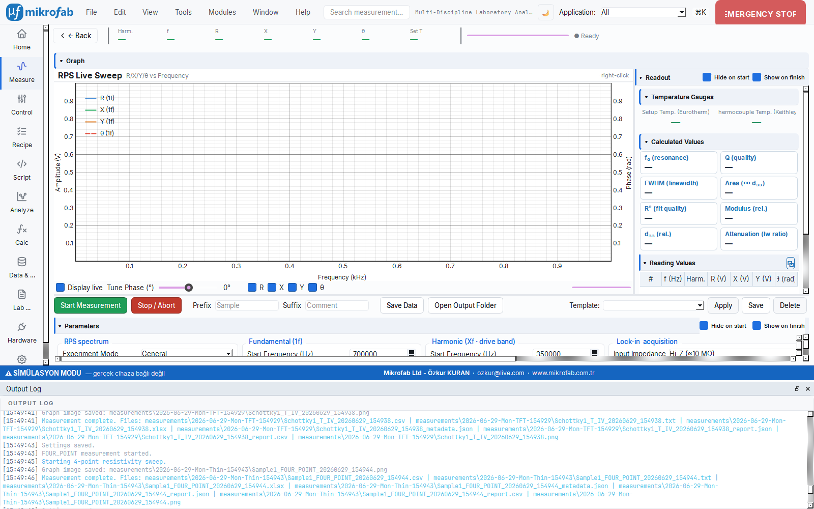
Resonance, quality factor and elastic tensor

The resonant piezo/acoustic spectroscopy (RPS) workstation scans mechanical resonance by sweeping the drive frequency, using a lock-in amplifier, an oven controller and a sample thermometer. It supports harmonics, temperature and stress as axes. At the end of a run a Lorentzian is fitted to the 1f spectrum; the analysis family (29–35) extracts resonances, acoustic damping, relative elastic modulus and the full elastic tensor (C_ij) from it.

Lorentzian fit. Resonance frequency f₀ (kHz), quality factor Q = f₀/FWHM, line width FWHM and peak area (∝ d₃₃ piezo coefficient).
Temperature-resolved. Acoustic damping Q⁻¹ ∝ FWHM(T), relative d₃₃, relative elastic modulus (f₀² ∝ c_eff/ρ) and nonlinearity ratio (Xf/1f).
Multi-mode (RUS). Complex (X/Y) two-pole fit to all resonances in the sweep; removes feedthrough-induced Fano asymmetry and gives unbiased f₀/Q.
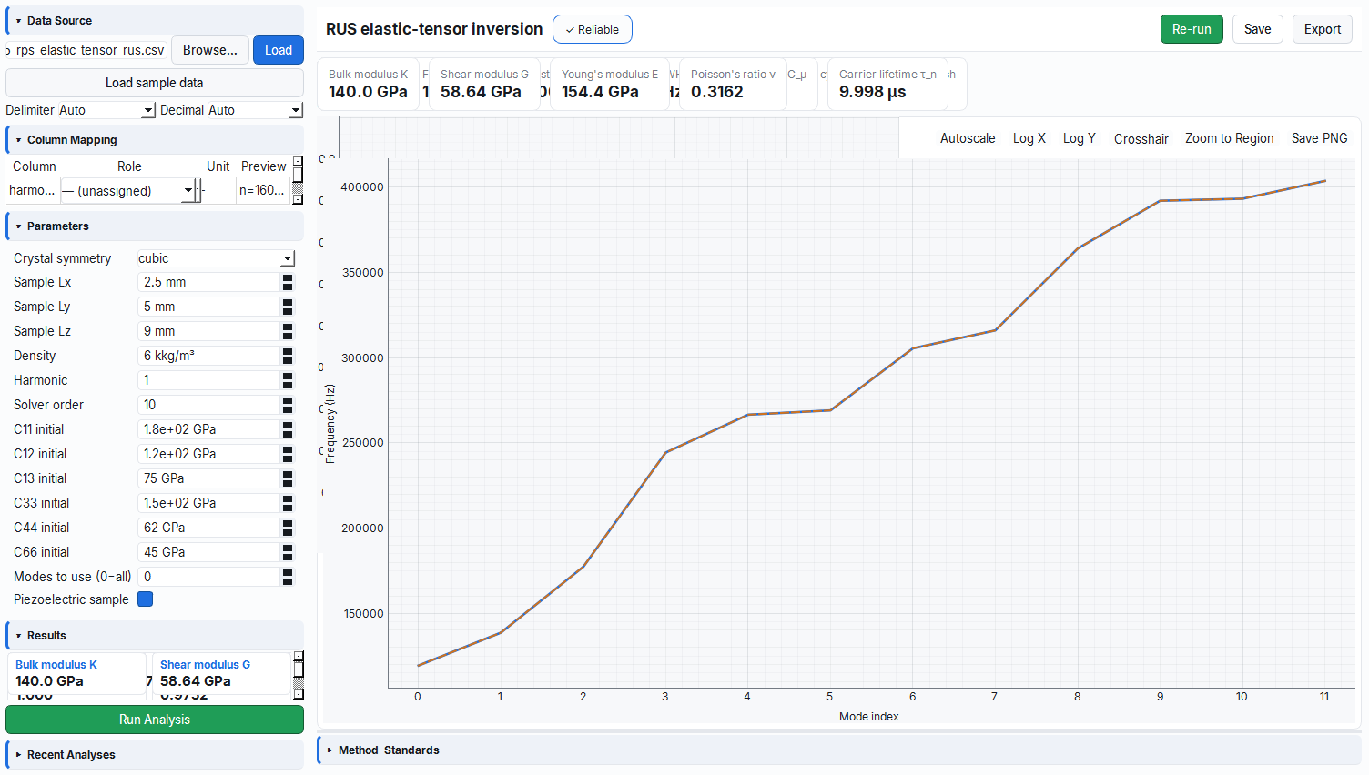
Elastic tensor inversion. The independent C_ij constants of the chosen crystal symmetry from a sample of known geometry + Voigt–Reuss–Hill aggregate moduli (K, G, E, ν) and Zener anisotropy.

Read about RPS / RUS

RESONANCE

f₀ · Q · FWHM · Area

Resonance frequency, quality factor, half-height line width and peak area from a high-Q Lorentzian fit; uncertainties are propagated with GUM from the fit covariance.

LorentzianV·Hz∝ d₃₃

ELASTIC TENSOR

C_ij · K, G, E, ν

Independent elastic constants are inverted from the measured multi-mode spectrum via the Rayleigh–Ritz / Visscher forward problem; five symmetry classes from isotropic to orthorhombic.

RUSVRHZener A

PHASE TRANSITION

Modulus · d₃₃ · damping

By tracking f₀², peak area and FWHM with temperature: elastic softening, relative piezoelectric response and anelastic loss; clearly reveals phase transitions.

modulus_relQ⁻¹≥2 temperatures

FAMILY 5 · PHOTODETECTOR

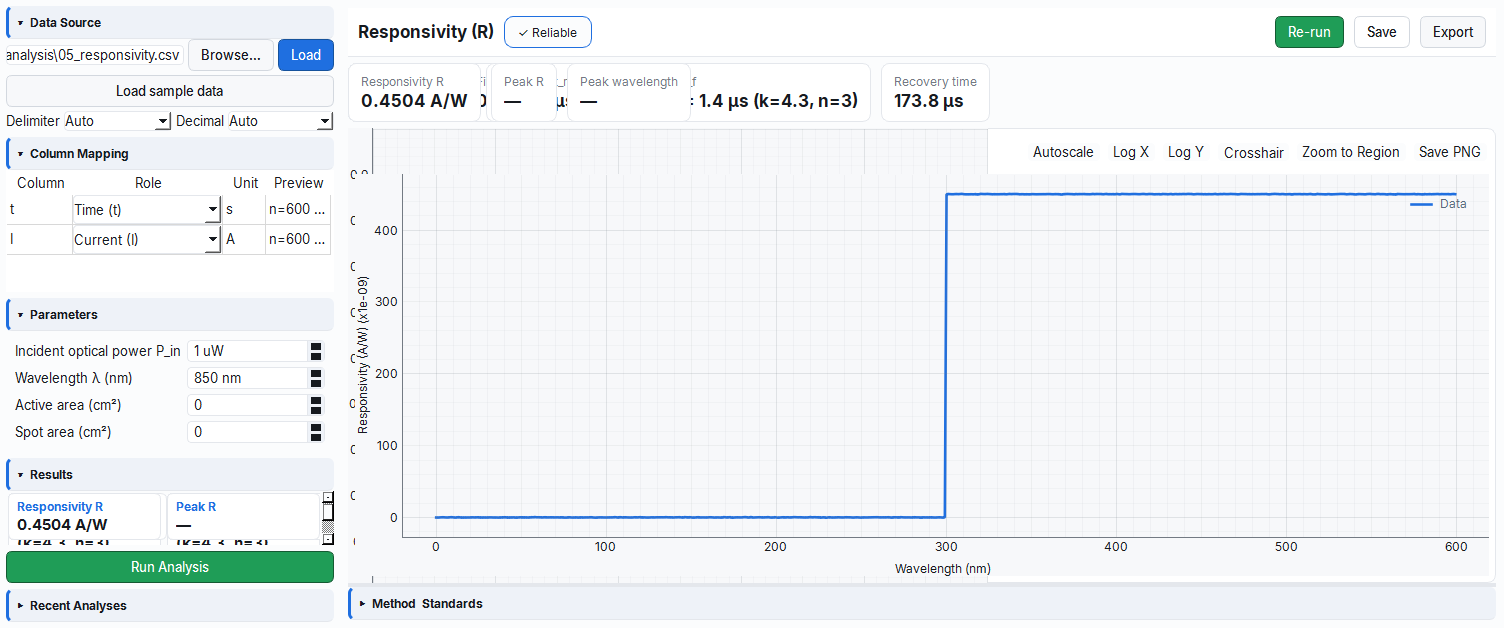
Responsivity, EQE, D* and rise time

The photodetector analysis family (Modules 1–10) extracts a complete performance package from photo-switching time series and dark-current noise. From spectral responsivity to quantum efficiency, from noise-equivalent power to specific detectivity, every metric is presented with its standard reference and a reliability badge. Roles are mapped automatically; files from different instruments are computed without manual mapping.

Spectral responsivity. Responsivity R = I_photo/P_det [A/W] and implied EQE = R·1239.84/λ; an R(λ) curve if a wavelength table is available (IEC 60904-8).
Quantum efficiency. External (EQE) and internal (IQE = EQE/(1−R_refl)) quantum efficiency; a gain-suspicion warning when exceeding 100%.
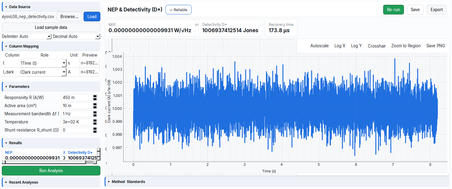
Noise & detectivity. NEP [W/√Hz], specific detectivity D* [Jones], dominant-noise (shot/thermal) discrimination and the 1/f^γ corner frequency from the noise PSD.
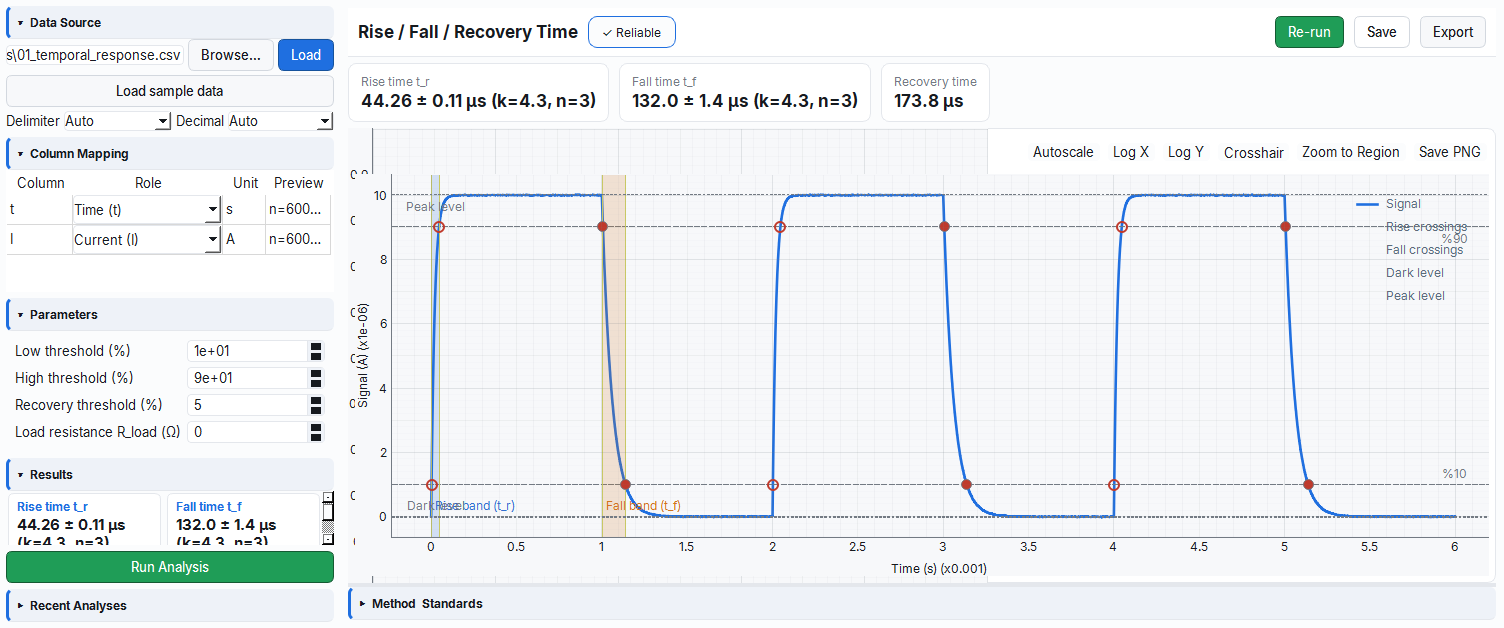
Temporal response. Rise/fall/recovery times (IEEE 181, IEC 60469), -3 dB bandwidth BW = 0.35/t_r, photo/dark ratio, SNR and linear dynamic range LDR.

Read about photodetector analysis

Photodetector spectral responsivity analysis: responsivity computed from incident optical power, implied EQE and the R(λ) curve versus wavelength

Metric	Symbol	Unit	Formula / Method
Spectral responsivity	R	A/W	I_photo / P_det
External quantum efficiency	EQE	%	R · 1239.84 / λ[nm]
Specific detectivity	D*	Jones	R · √(A·Δf) / i_noise
Noise-equivalent power	NEP	W/√Hz	noise density / R
Rise time	t_r	s	10% → 90% transition (IEEE 181)
-3 dB bandwidth	BW	Hz	0.35 / t_r
Linear dynamic range	LDR	dB	20·log₁₀(P_max/P_min); power law α (IEC 60904-10)

ANALYSIS GALLERY

Extracted metrics, real analysis screens

Every analysis module is validated against a physics-based synthetic “ground truth” data set; the numbers in the manual are reproducible bit for bit in the product. The screens below were produced with the shipped sample data sets.

Solar cell J-V metrics analysis: Voc, Jsc, FF, PCE, Rs and Rsh values with the J-V curve — Solar cell J-V metrics: J_sc=30 mA/cm², V_oc≈0.696 V, FF≈0.755, PCE≈15.8%.

TFT transfer analysis: on/off ratio, threshold voltage Vth and subthreshold swing SS with the transfer curve — TFT transfer (on-off): I_on/I_off≈10⁸, V_th≈0.75 V, SS≈345 mV/dec.

Mott-Schottky analysis: the 1/C² - V line, carrier density Neff and built-in voltage Vbi — Mott-Schottky: c-Si sharp junction, N_eff≈10¹⁶ cm⁻³, V_bi≈0.70 V.

RUS elastic tensor inversion: cubic crystal C11, C12, C44 constants and VRH aggregate moduli — Elastic tensor (RUS): cubic C11≈200, C12≈110, C44≈70 GPa; Zener A≈1.56.

NEP and detectivity analysis: specific detectivity D* from dark-current noise and the dominant noise mechanism — NEP & detectivity: D*≈10¹² Jones for a realistic Si photodiode.

Advanced J-V report: sign convention, forward/reverse hysteresis, dynamic metrics and kink/S-shape diagnostics — Advanced J-V report (Spec v2.0): hysteresis, dynamic metrics and diode diagnostics.

Temporal response analysis: rise, fall and recovery times from a photo-switching series — Temporal response: single-pole RC, t_rise=43.9 µs, t_fall=131.8 µs.

Impedance Nyquist fit: Rs, Rrec, Cmu and carrier lifetime from the Randles equivalent circuit — Impedance (Nyquist) fit: R_s≈5 Ω, R_rec≈5 kΩ, τ_n≈10 µs.

✅

Single-source principle. The measurement side and the analysis side share the same core engine (e.g. transfer, diode and PV metrics). You can later load the data you measured into the Analysis workspace and re-validate the same metrics, or re-evaluate them with different fit ranges — there is no metric drift.

LEARN AND APPLY

Get started with training, the manual and examples

Don't just read about the capabilities; run your own measurement in simulation mode, load the shipped sample data sets into the Analysis workspace and learn the physics behind every metric with the step-by-step manual.

Professionals

R&D and production laboratories

Bring five families to a single bench and tie them to a traceable, sealed report
High-volume scanning across the wafer with a Switch Matrix + recipe
A reliability gate with bias-stress, endurance and degradation
A record ready for audit and accreditation with standard-cited outputs

Academia

Researchers, students and education

Risk-free learning and classroom demos with hardware-free simulation mode
Correct methodology with GUM uncertainty + reliability badge
Reproduce every metric with validated sample data sets
Advanced characterization techniques from Mott-Schottky to the elastic tensor

📘

User manual

Measurement and analysis catalogs, formulas and standard bases, step by step. A separate section for each family.

Open the manual

🎓

Academy

Method-based training content: V_th extrapolation, fill factor, Mott-Schottky and more.

Go to the Academy

🧪

Solutions

Which measurement family for which instrument/material? Capability mapping by application scenario.

See the solutions

Try the capabilities with your own data

Mikrofab Suite runs without hardware in simulation mode; you can explore all 37 measurement modes and 37 analysis modules right up to installation. Request a personalized demo or start right away with the manual.

Request a demo Open the user manual

Measurement & Analysis Capabilities