LCR, RPS, DMM and Temperature/Control

This chapter covers the four specialized workstations of the Mikrofab measurement software: LCR/Impedance (capacitance–voltage, capacitance–frequency, impedance spectroscopy, Mott–Schottky and temperature-resolved admittance sweeps), RPS (resonant piezo/acoustic spectroscopy), DMM Monitor (time-dependent live monitoring with a multi-function bench multimeter) and the Temperature/Control family (Set-Point voltage/current profiling and furnace-based Temperature Profiling). Each module is hosted inside exactly the same composite measurement frame as the transistor/diode panels: parameter panel on the left, live plot in the center, live readout panel on the right; with the shared Start / Stop / Save action bar at the bottom.

ℹ️

Note All modules run mock-first (simulation-first). When no hardware is connected, each panel generates realistic synthetic data and an orange ⚠ Demo badge is shown in the top header bar. For a real measurement, select the corresponding instrument and VISA/port address.

🎓 What is it for? — This chapter: LCR, RPS, DMM and Temperature/Control

This chapter describes four different ways of "electrically listening" to a material or a device. Just as a physician sometimes checks a patient's pulse (DMM), sometimes runs an ECG (LCR/impedance), and sometimes performs a vibration test with a tuning fork (RPS), each workstation asks the sample a different "question"; you can think of it as connecting different diagnostic instruments to the same patient. The Temperature/Control modules, in turn, drive the voltage applied to the sample or the furnace temperature in a programmed manner over time.

Why it is done: to learn a sample's capacitance, resistance, mechanical resonance, or how these quantities change with temperature, and thereby infer something about its internal structure.
What it teaches / measures: it measures or applies quantities such as impedance, capacitance, resonance frequency, live readout values and applied temperature/voltage profiles.
Where it is used: semiconductor / solar cell research, materials characterization, quality control and failure analysis.

1. LCR / Impedance Workstation

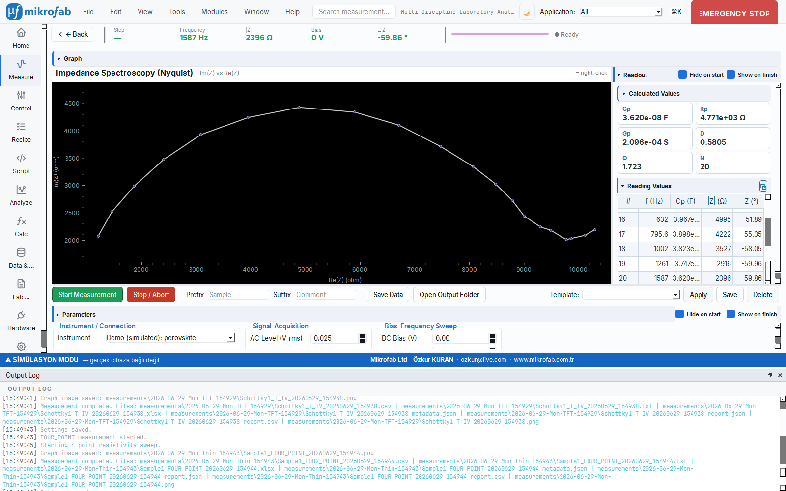
🎓 What is it for? — LCR / Impedance Workstation

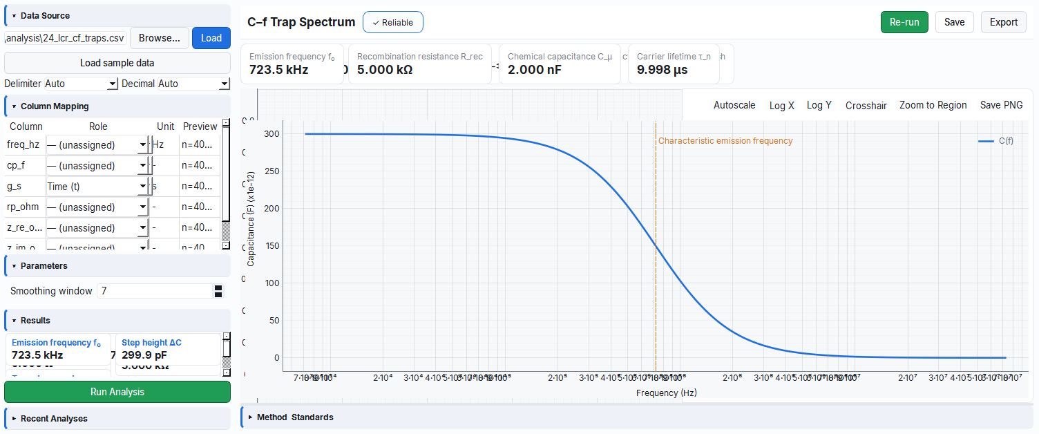
An LCR/impedance measurement applies a small alternating (AC) signal to the sample and measures "how much it resists" (its impedance); that is, it determines whether the material behaves more like a capacitor or more like a resistor. It is like gently vibrating a guitar string and listening to its response: it reveals the sample's capacitance and resistance at different DC voltages and frequencies. With plots such as Mott–Schottky, invisible physical quantities such as doping density and built-in voltage are also computed.

Why it is done: to understand the charge distribution, the depletion region and the trap (defect) states in a semiconductor junction.
What it teaches / measures: capacitance (C), impedance (Z), dissipation/quality factor (D/Q), and the doping density (N) and built-in voltage (V_bi) derived from them.
Where it is used: solar cell/diode research, materials characterization and defect (trap) analysis.

Navigation key (nav_key): lcrws. The LCR module has a different execution path from the classic SMU measurements: its own LCR driver (not an SMU), its own LcrPvMeasurement runner, and it returns a Dataset instead of a (point, summary) pair. The panel gathers four measurement modes into a single form and shows the relevant field group according to the selected mode.

LCR / Impedance workstation: mode and sweep parameters on the left, live impedance plot in the center, calculated values panel on the right — **Figure.** LCR / Impedance workstation — a composite measurement frame gathering the four measurement modes (C-V, C-f, Z-f, TAS) into a single form.

1.1 Measurement Modes

Mode	Code	Held fixed	Swept	Live plot
C-V (capacitance–voltage)	`cv`	Frequency	DC bias	C vs Bias
C-f (capacitance–frequency)	`cf`	DC bias	Frequency (log)	C vs f (log-x)
Z-f (impedance spectroscopy)	`zf`	DC bias	Frequency (log)	Nyquist (−Im Z vs Re Z)
TAS (temperature-resolved admittance)	`tas`	DC bias	Frequency + Temperature	C vs f (for each T)

✅

Tip In Z-f mode the plot is drawn as a Nyquist diagram (with locked equal aspect ratio); the semicircles appear with their true geometry. In C-f and TAS modes the frequency axis is logarithmic.

1.2 Connection and Instrument

Parameter	Unit	Description	Default
Instrument	—	`Demo: <preset>` (5 simulations) or a real `E4980A` / `BK894`	Demo
VISA address	—	Enabled only with a real instrument (e.g. `USB0::0x0957::...::INSTR`)	(empty)
Mode	—	cv / cf / zf / tas	zf

Simulation presets: perovskite, c_si, cigs, iii_v, opv. Real drivers: Keysight E4980A and B&K Precision BK894 (connected over the VISA transport).

1.3 Signal (Excitation) Parameters

Parameter	Unit	Range	Description	Default
AC level	V rms	0.005 – 0.1	Small-signal excitation amplitude	0.025
Area	cm²	1e-4 – 100	Sample active area (for density-derived quantities)	0.09
Averaging	count	1 – 16	Number of averages per point	4
Settle	s	0 – 10	Wait before each point	0.5

⚠️

Warning If the AC level is set too high, the small-signal (linear) assumption breaks down; when the threshold is exceeded the panel shows an inline warning message (ac_level_warning) under the field.

1.4 Sweep Parameters (by mode)

C-V (cv) group

Parameter	Unit	Range	Default
Frequency (fixed)	Hz	1e3 – 1e6	100000
Bias start	V	−40 – 40	−1.0
Bias stop	V	−40 – 40	0.5
Bias step	V	0.005 – 5.0	0.02

C-f / Z-f / TAS frequency group

Parameter	Unit	Range	Default
Bias (fixed)	V	−40 – 40	0.0
f_min	Hz	0.01 – 1e6	20.0
f_max	Hz	1.0 – 2e6	1e6
Points per decade (ppd)	count/decade	1 – 40	10

TAS temperature group (tas only)

Parameter	Unit	Range	Default
T start	K	4 – 400	150.0
T stop	K	4 – 400	350.0
T step	K	1 – 100	10.0

ℹ️

Note Validation (ADR 0010 D9): in C-V mode bias_start ≠ bias_stop and in frequency sweeps f_min < f_max must hold; otherwise Start is blocked and an inline error message is shown.

1.5 Read and Derived Quantities

Each point carries the raw complex impedance (z_re, z_im). The readout panel on the right and the live plot derive the parallel-equivalent circuit quantities from the raw impedance (not the heavy P14 analysis engine; a single-source lightweight formula):

ω   = 2·π·f
|Z| = hypot(z_re, z_im)
∠Z  = atan2(z_im, z_re)        [degrees]
Y   = 1/Z = (z_re − j·z_im) / |Z|²
Gp  = Re(Y) = z_re / |Z|²       [S]   (parallel conductance)
Bp  = Im(Y) = −z_im / |Z|²
Cp  = Bp / ω                    [F]   (parallel capacitance)
Rp  = 1 / Gp                    [Ω]   (parallel resistance)
D   = Gp / Bp                          (dissipation factor)
Q   = 1 / D                            (quality factor)

The Calculated Values section of the readout panel live-updates the Cp / Rp / Gp / D / Q cards plus a point counter (n). The Read Values table accumulates, row by row, the x-axis (bias in C-V, frequency otherwise) and the Cp / |Z| / ∠Z columns according to the mode; the ⧉ button in the header opens the readout list in a floating window.

Quantity	Symbol	Unit	Source
Parallel capacitance	Cp	F	Im(1/Z)/ω
Parallel resistance	Rp	Ω	1/Gp
Parallel conductance	Gp	S	Re(1/Z)
Dissipation factor	D	—	Gp/Bp
Quality factor	Q	—	1/D
Impedance magnitude	\|Z\|	Ω	hypot(z_re, z_im)
Impedance phase	∠Z	°	atan2(z_im, z_re)

1.6 Mott–Schottky and Physics Basis

The simulation is based on sound physics models (analysis_kit/sim). C-V mode produces the depletion capacitance via the Mott–Schottky relation:

Formula C_dep(V) = ε·A / W W = sqrt( 2·ε·(V_bi − V) / (q·N) )

Here ε = εr·ε0 (dielectric permittivity), A is the area, V_bi is the built-in voltage, N is the effective doping, and q is the electron charge. N is extracted from the slope of the 1/C² – V plot and V_bi from its axis intercept (standard Mott–Schottky analysis). The bias is clamped above V_bi − 0.05 V (to prevent the W→0 blow-up).

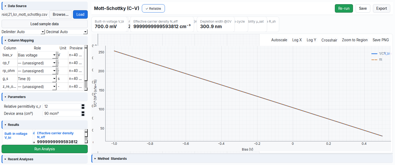
Mott-Schottky analysis: linear segment of the 1/C-squared curve versus bias, doping extracted from the slope and built-in voltage from the intercept — **Figure.** Mott–Schottky analysis — the effective doping N is derived from the slope of the `1/C²` – V plot and the built-in voltage V_bi from the axis intercept.

In C-f / TAS mode the capacitance is the sum of the geometric capacitance + trap Debye contributions + Urbach band-tail:

C(ω) = C_geo + Σ_i  dC_i / (1 + (ω/ω_i)²)
ω_i(T) = 2·ν0·T²·exp(−E_i / kT)         (trap characteristic frequency)

Z-f mode produces the equivalent-circuit impedance: R_s − (R_tr‖C_geo) − (R_rec‖C_mu or CPE) − (low-f Warburg). This physics mimics the behavior of real perovskite/c-Si/CIGS/III-V/OPV devices.

C-f trap analysis: Debye steps and trap characteristic frequencies extracted from the variation of capacitance with frequency — **Figure.** C-f trap analysis — trap Debye contributions and characteristic frequencies are resolved from the capacitance-frequency steps.

1.7 Mock Behavior

The simulated LCR meter (SimulatedLcrMeter) runs the selected preset with noise_rel = 0.005 (0.5% relative noise). It is deterministic: the same seed → the same sequence; in noiseless mode (noise_rel=0) it returns the exact analytical value. Saving: the Save button writes the last Dataset to disk with the composite prefix/suffix (save_dataset). The sim generators (generate_cv/cf/zf/tas) are pure NumPy; they run without Qt and without SCPI, and they also feed the golden tests of the Analysis module.

2. RPS — Resonant Piezo / Acoustic Spectroscopy

🎓 What is it for? — RPS — Resonant Piezo / Acoustic Spectroscopy

RPS applies a vibration (a drive signal) to the sample and searches for the resonance frequency at which it "rings" most strongly; it is like tapping the rim of a glass and finding the note at which it rings most beautifully. The position and sharpness of this resonance reveal information about the material's stiffness (mechanical modulus) and piezoelectric strength (d₃₃). Moreover, by tracking how this resonance shifts as the temperature changes, phase transitions can be studied.

Why it is done: to quantify a material's mechanical resonance and its piezoelectric/electrostrictive behavior as a function of temperature.
What it teaches / measures: the resonance frequency f₀, the quality factor Q, the linewidth FWHM, and relative changes in d₃₃ / modulus / damping.
Where it is used: piezoelectric/ferroelectric materials research and temperature-dependent phase-transition studies.

Navigation key: rpsws. RPS is a three-instrument measurement that works with a lock-in amplifier (Zurich Instruments MFLI), a furnace controller (Eurotherm or Sun EC10) and a sample thermometer (Keithley 2000). It scans the piezoelectric/electrostrictive mechanical resonance by sweeping the drive frequency; it supports harmonics, temperature and voltage as axes. The panel presents seven cards + two collapsible sections (Temperature Profile, Voltage Profile) in a masonry (responsive card) layout that mirrors the legacy LabVIEW front panel.

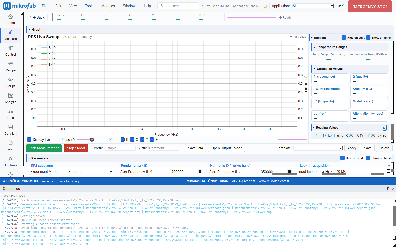
RPS resonant piezo/acoustic spectroscopy workstation: mode, frequency, lock-in and temperature controls in a masonry card layout — **Figure.** RPS workstation — a masonry layout mirroring the legacy LabVIEW front panel; a three-instrument (lock-in + furnace + thermometer) resonance scan.

2.1 Mode Controls

Parameter	Options	Description
Experiment mode	GENERAL / VOLTAGE / TIME	Outer sweep axis: T only / T→V / fixed (repeated)
Spectrum mode	1f / Xf / 1f&Xf	Harmonic selection: fundamental / harmonic X / both
Harmonic X	2 – 10	Harmonic index of the Xf channel (default 2)
Drive amplitude	0 – 10 Vpp	Fixed excitation in GENERAL/TIME mode (default 1.0)

ℹ️

Note GENERAL sweeps temperature only; VOLTAGE sweeps voltage within temperature (requires at least one Voltage Segment); TIME repeats time_repeats times at a fixed (T, V) point.

2.2 Frequency Controls (1f and Xf independent)

Each harmonic channel has its own frequency configuration (FreqConfig):

Parameter	Unit	Range	1f default	Xf default
Start	Hz	1e4 – 5e6	700000	350000
Stop	Hz	1e4 – 5e6	900000	450000
Number of points (n_points)	count	2 – 100000	4000	4000
Time constant (tc)	s	1e-4 – 10	0.030	0.030
Input range (range)	V rms	1e-7 – 10	300e-6	300e-6
Auto-TC (auto_tc)	—	on/off	off	off

✅

Tip Xf "drive band": Detection is at harmonic_x × drive frequency; therefore, to probe the same mechanical resonance (700–900 kHz) on the 2f channel, the drive is swept at 350–450 kHz (2× = 700–900). This default is editable.

2.3 Lock-in and Temperature

Parameter	Options / Range	Default
Input impedance	50 Ω / Hi-Z (≈10 MΩ)	Hi-Z
Differential input (diff)	on/off	on
Temperature stage	YDG-1206 (30…1200 °C) / LMS3620 (−180…500 °C) / EC10 (−184…315 °C)	YDG-1206
Return to room temperature at end	on/off	off
Stay duration (stay)	min (0–480)	0
Time repeats (time_repeats)	1 – 9999	1
Wait between scans	s (0–3600)	0
Rotate phase (rotate_phase)	on/off	off
Tune phase (tune_phase)	° (−180…+180)	0

2.4 Temperature Profile (segment table)

The Temperature Profile section contains the global ramp/settle parameters + the segment table + the preview plot + the summary statistics.

Global parameter	Unit	Range	Default
Ramp	°C/min	0.1 – 100	5
Settle	s	0 – 3600	30
Tolerance (tol)	°C	0.1 – 50	1
Settle source	Sample TC / Furnace PV	—	Sample TC

Each row is a temperature segment (start/stop/step, °C; table range −200…1300 °C, step 0.1…500). The number of set-points is derived as round(|stop − start| / step) + 1. The preview draws the segments as a staircase (each transition: ramp to the new set-point + flat settle); the summary boxes show the set-point count, the estimated duration and the temperature range.

ℹ️

Note Settle source selection (important): Sample TC (default) opens the gate when Keithley's sample thermocouple comes within tol_c of the set-point (more rigorous; waits for the real sample temperature). Furnace PV tracks the Eurotherm process value (faster; absorbs the furnace→sample thermal lag with the settle_s wait).

2.5 Voltage Profile (VOLTAGE mode only)

At most 9 voltage segments (start_v / end_v / step_v; range 0–10 V, step 0.001–5). Only the enabled (checked) segments are included in the plan. At each temperature step, the drive amplitude is swept across the start_v → end_v range with a step_v step.

2.6 Read Quantities and Phase Rotation

The lock-in produces four quantities at each point: R (amplitude), X and Y (quadrature components) and θ (phase, radians). The live plot is dual-axis: the left axis is Amplitude (V) — the R/X/Y traces; the right axis is θ (rad). The 1f traces are solid, the Xf traces are dashed; Xf is drawn only when the spectrum mode includes Xf.

Tune-phase rotation rotates the display phase without corrupting the data (M-5 two-buffer; the raw data is stored, and the display is rebuilt on each change):

X' =  X·cos(φ) − Y·sin(φ)
Y' =  X·sin(φ) + Y·cos(φ)
θ' =  atan2(Y', X')
R' =  hypot(X', Y')

Above the plot there is a −180…+180° slider, R/X/Y/θ toggle boxes, a "show while measuring" switch and a progress bar.

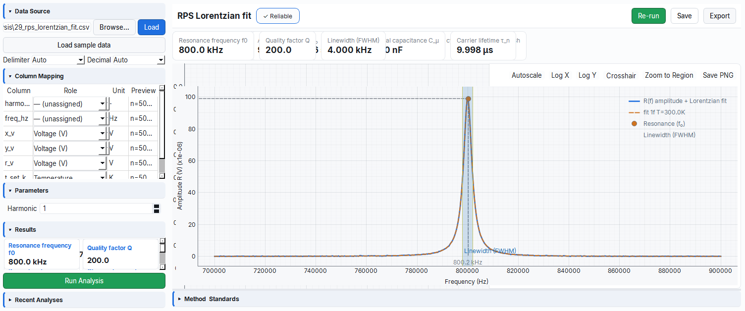
2.7 Calculated Metrics (end-of-run Lorentzian fit)

When the run finishes, a Lorentzian is fitted to the 1f spectrum and summary metrics are computed (compute_live_metrics):

f₀ResonancekHz

Qf₀/FWHM—

FWHMLinewidthkHz

APeak areaV·Hz

R²Fit quality—

Metric	Symbol	Unit	Description
Resonance frequency	f₀	kHz	Lorentzian peak position
Quality factor	Q	—	f₀ / FWHM
Linewidth	FWHM	kHz	Full width at half maximum
Area	A	V·Hz	Area under the peak (∝ d₃₃ piezo coefficient)
Goodness of fit	R²	—	Fit quality
Modulus (relative)	—	—	Temperature-relative (in runs with ≥2 T)
d₃₃ (relative)	—	—	Temperature-relative (in runs with ≥2 T)
Damping	—	—	Temperature-relative (in runs with ≥2 T)

The last three metrics require at least two temperature runs; at a single temperature they show "—". The right panel also has a Temperature Indicators (furnace PV + sample TC) section.

RPS Lorentzian fit analysis: curve fitted to the resonance peak, extraction of resonance frequency, FWHM and quality factor — **Figure.** End-of-run Lorentzian fit — the f₀, FWHM, Q and area-under-the-peak (∝ d₃₃) metrics are extracted from the 1f resonance peak.

2.8 Duration Estimate, Mock and Validation

Duration estimate (Refresh button):

Formula sweep_s = n_point × (tc×5 + 0.010 s) (×2 if spectrum is BOTH) total = n_temperature × n_voltage × n_repeat × sweep_s

Mock behavior: If all three instruments are simulated, a BaTiO₃-like physics model (RpsSimModel) + a live sample-temperature provider is attached to the lock-in; the spectra evolve with temperature and drive amplitude (field-driven RPS). In a simulated sweep, a delay of ~2 ms per point is added, so the mock run plot comes alive point-by-point (a 4000-point sweep is drawn in ~8 s). The simulated furnace PV jumps instantly to the set-point (it does not wait for a real-minutes ramp); the sample TC tracks the furnace with a short delay.

⚠️

Warning Validation (Pydantic): drive_vpp ≤ 10 Vpp (MFLI output limit); segment counts ≤ 9; VOLTAGE mode requires ≥1 voltage segment; start_hz < stop_hz for each channel; all planned temperatures within the selected stage limits. With an invalid plan, Start is disabled and an inline error is shown.

3. DMM Monitor — Live Readout and Logging

🎓 What is it for? — DMM Monitor — Live Readout and Logging

The DMM Monitor is a "data recorder" that keeps a multimeter (a bench instrument that measures voltage, current, resistance, temperature...) continuously on and logs its readings over time. It is like connecting a patient's pulse to a monitor and watching it for hours: it shows how a single quantity changes over time with a live plot and statistics. If you wish, you can set a pass/fail band and have it automatically check whether the value goes out of bounds.

Why it is done: to monitor the stability, drift or noise of a signal (voltage, current, temperature...) over time.
What it teaches / measures: the instantaneous value of the selected function and live statistics such as min/max/mean/standard deviation.
Where it is used: long-term stability tests, quality control and laboratory monitoring/logging.

Navigation key: dmmmon. The DMM Monitor performs time-dependent continuous monitoring + logging with a multi-function bench multimeter (or an SMU's "DMM duty"). The panel is a semi-skeuomorphic "virtual front panel" that gives the feel of a real instrument: a keypad (function/range/speed/time/limit) on the left, and on the right a readout panel with a large "7-segment" display + live statistics.

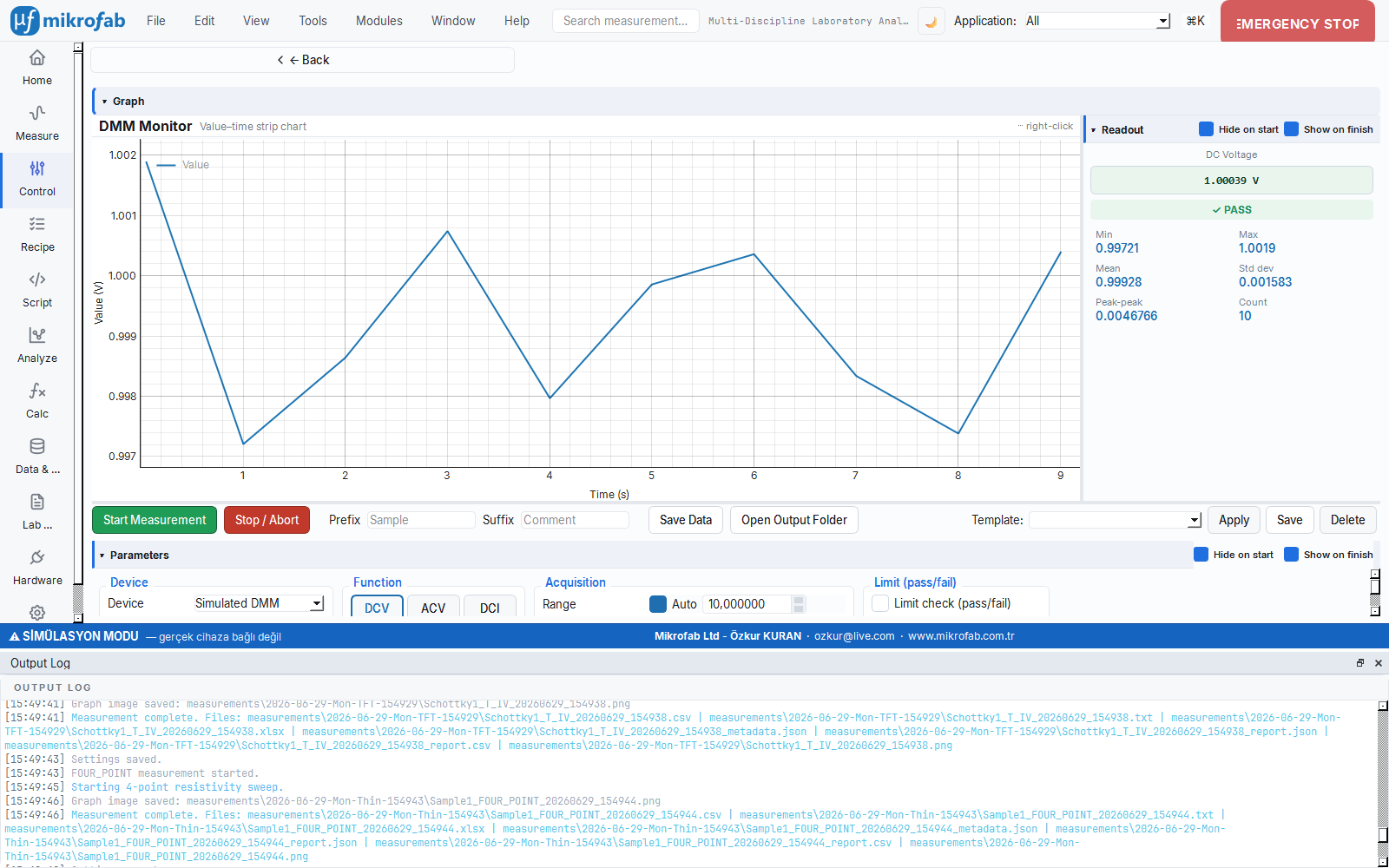
DMM Monitor virtual front panel: function keypad on the left, large 7-segment display and live statistics grid on the right — **Figure.** DMM Monitor — a semi-skeuomorphic virtual front panel; time-dependent continuous monitoring and logging.

3.1 Functions

Twelve mutually-exclusive function keys (like the instrument's own function keys):

Key	Function	Key	Function
DCV	DC voltage	Period	Period
ACV	AC voltage	Temp	Temperature
DCI	DC current	Cont	Continuity
ACI	AC current	Diode	Diode
2W	2-wire resistance	Cap	Capacitance
4W	4-wire resistance	Freq	Frequency

Default: DCV. Functions not supported by the selected instrument are disabled.

3.2 Range, Speed and Time

Parameter	Unit	Range	Default
Autorange	—	on/off	on
Manual range	(by function)	1e-6 – 1e9	10
Speed (NPLC)	—	Fast=0.1 / Medium=1.0 / Slow=10.0	Medium (1.0)
Sampling interval (interval)	s	0.02 – 3600	1.0
Indefinite	—	on/off (∞)	on
Duration	s	0.1 – 1e6	60

✅

Tip When "Indefinite" is checked, logging runs without limit (the opposite of BenchVue's 1-hour limit); since statistics are kept incrementally, memory does not balloon. NPLC is the integration time: higher NPLC = less noise, slower reading.

3.3 Limit Band (Pass/Fail)

Parameter	Unit	Range	Default
Limit enabled	—	on/off	off
Low limit (low)	(function unit)	−1e9 – 1e9	−1.0
High limit (high)	(function unit)	−1e9 – 1e9	1.0

When the limit is enabled, low/high lines + a green pass-band in between are shown on the live plot; the readout panel lights a ✓ PASS / ✕ FAIL badge at each sample. When the band is exceeded, a limit_violated warning appears in the status bar.

3.4 SMU "Voltmeter Duty"

A source-measure unit (SMU/PSU) selected from the inventory can be used like a DMM. In the voltage function the SMU forces 0 A; with an open input, the reading drifts to ±compliance. For this reason, when an SMU is selected the panel shows a compliance/range (V) field (0.2–200 V, default 2.0) and, in the voltage function, an amber open-input warning. A low compliance limits this drift and puts the SMU into a low-noise range.

3.5 Read Quantities and Statistics

The readout panel shows the large instantaneous value (function + unit); on overflow it shows OL (overload). Below it is an incremental statistics grid using the Welford algorithm:

Statistic	Symbol	Description
Min / Max	—	Smallest / largest reading
Mean	x̄	Run mean (incremental)
Std deviation	σ	Standard deviation (Welford)
Peak-to-peak	p-p	max − min
Count	n	Total number of samples

The live plot is a single-trace strip-chart (value vs elapsed time); pyqtgraph applies an SI prefix for the unit (mV/µA/kΩ…). Overflow readings are not fed into the trace; they are shown with a separate red "×" marker.

ℹ️

Note Mock behavior: The static list shows only the Simulated DMM (SIM); real instruments come from the live inventory (with the measure_v capability + connected/IDLE state). When SIM is selected, SimulatedMultimeter generates a synthetic value appropriate to the function. Save writes the readings to CSV; the first two columns are elapsed_s + timestamp (each file is self-describing — a zero-setup origin).

4. Set-Point Profile (Voltage/Current Control)

🎓 What is it for? — Set-Point Profile (Voltage/Current Control)

The Set-Point Profile drives the output of a power supply or an SMU over time according to a recipe you draw in advance: "rise from 0 V to 10 V over so many seconds, hold for a while, then come back down". It is like setting a timer on an oven and changing the temperature in stages, but here for electrical voltage/current. At the same time it live-reads and records the sample's response (e.g. the current flowing in response to the driven voltage).

Why it is done: to stress the sample with a controlled, repeatable voltage/current program and observe its response (e.g. stress testing, aging).
What it teaches / measures: the applied set-point, the instrument's read-back, the other measured quantity (V↔I) and the derived resistance R = V/I.
Where it is used: endurance/stress tests, controlled supply scenarios and production/quality flows.

Navigation key: profile. The Set-Point Profile is a control module that drives a source (PSU or SMU) over time along a programmed voltage/current profile (ramp + hold) while reading simultaneously. The left panel has the instrument, the program table, the options and the live preview; the right has the live readout.

Figure. Set-Point Profile — a control module that drives a source along a programmed voltage/current profile (ramp + hold).

4.1 Instrument and Quantity

Parameter	Options	Description
Instrument	Simulated PSU (SIM) / SMU / inventory instruments	In simulation only SIM; real ones from the live inventory
VISA address	—	Enabled only for a manually-addressed static PSU
Channel	1 – 3	For multi-channel PSU (hidden for SMU)
Quantity	Voltage / Current	The driven quantity (a V profile reads I; an I profile reads V)
Time unit	s / min / h	Program table time scale

ℹ️

Note The instrument list shows only the simulation source + the instruments in the live inventory that are connected and have the source_v capability; an instrument that is not auto-discovered appears in the list automatically once it is added and verified from the Hardware page.

4.2 Program Table

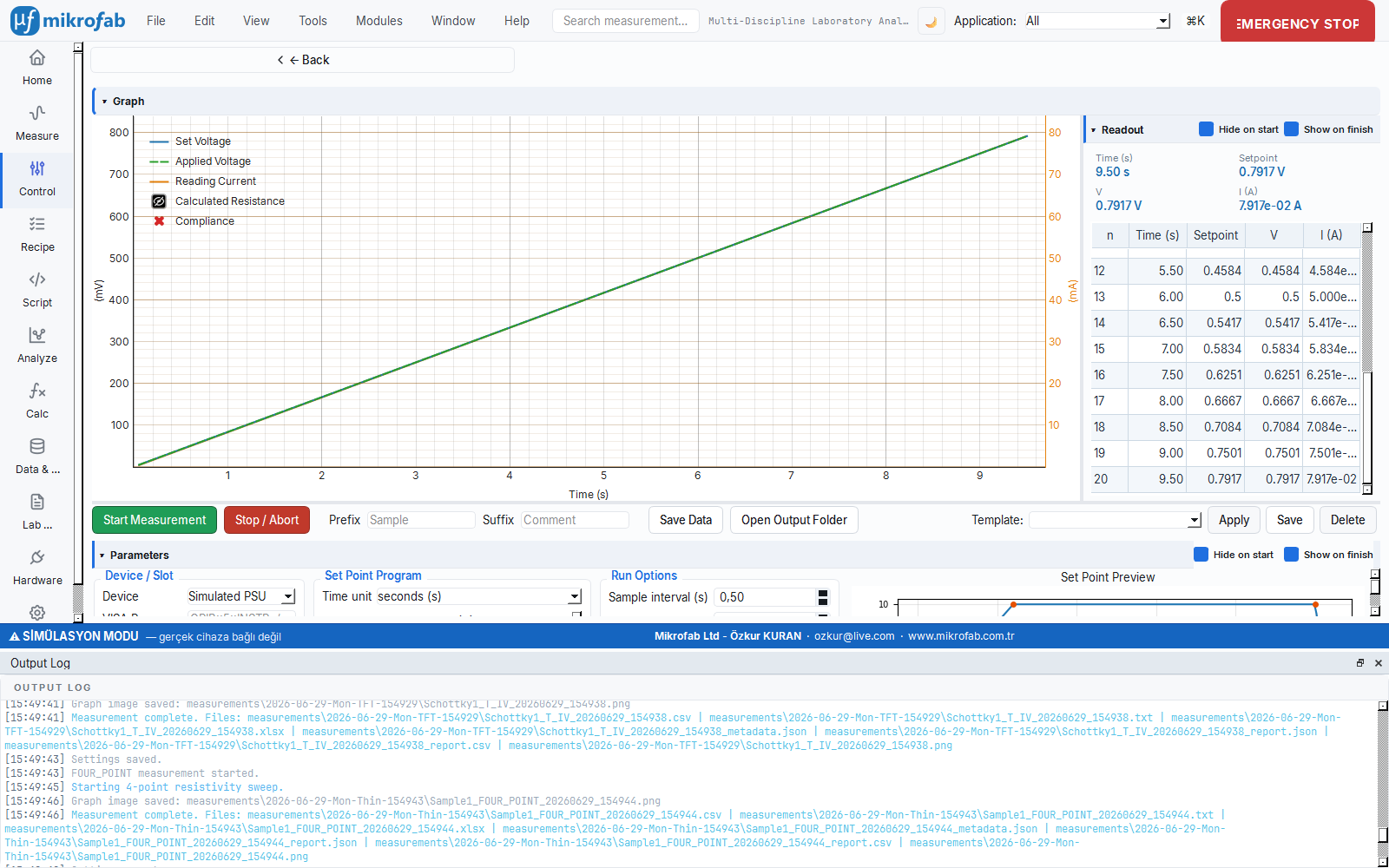
Each row is a breakpoint: (time, target, interpolation). The interpolation is ramp (linear transition between points) or step. The default voltage program:

Time (s)	Target (V)	Interp
0	0.0	ramp
120	10.0	ramp
500	10.0	ramp
520	0.0	ramp

The target column rescales according to the quantity: voltage −60…60 V (3 decimals), current −6…6 A (5 decimals). The preview draws the profile with 200 samples (setpoint_at) and shows the breakpoints with orange markers.

4.3 Options

Parameter	Unit	Range	Default
Sampling interval	s	0.01 – 3600	0.5
Settling	s	0 – 100	0.05
NPLC	—	0.01 – 100	1.0
Current/Voltage limit	A or V	0 – 1000	0.1 (V profile) / 20 (I profile)
Power limit	W	0 – 1000	20.0
Hold last value (hold_last)	—	on/off	off

⚠️

Warning The limit label changes according to the quantity: when driving voltage you enter a current compliance, when driving current a voltage limit. When the instrument hits compliance (CC mode), the readout panel lights an amber "current-limit" badge and a red "×" marker is placed on the plot.

4.4 Live Plot (three-axis) and Readout

The profile plot has a single X (time) and three Y axes:

Left axis — the driven quantity: Set (command) + Applied (instrument read-back, if available).
Right axis — the other read quantity: Reading (I in a V profile, V in an I profile).
Far-right axis — Calculated Resistance R = V/I (Ω, hidden by default).

Compliance (CC) points are shown with separate red markers. All Y axes are aligned at a common 0 level; each trace can be toggled on/off from the right-click menu, and as you hover with the mouse a time line + all values inside a box are read (snap-to-data). The readout panel keeps four instantaneous cards (t / set-point / V / I) + a growing row table.

ℹ️

Note Mock + Save: When SIM is selected, make_power_supply sets up a simulated PSU. Save writes the measurement points of the last run to CSV (MeasurementPoint fields).

5. Temperature Profile (Furnace Control)

🎓 What is it for? — Temperature Profile (Furnace Control)

The Temperature Profile drives a furnace/temperature stage step by step according to a recipe: ramp up to a target at a certain rate (ramp), hold there for a while (soak), then move on to the next target. It is like programming a baking oven to "heat to 180 °C, bake for 30 min, then cool down". The software waits until the sample's real temperature gets close enough to the target (the settle tolerance) and only then advances; this way each step is reliable.

Why it is done: to expose the sample to a known, repeatable temperature history (annealing, preparation for temperature-dependent measurement).
What it teaches / measures: the target temperature, the measured process value (PV), the phase (ramp/soak) and the settle state — all over time.
Where it is used: heat treatment/annealing, temperature-resolved experiments and process validation.

Navigation key: tempprofile. The Temperature Profile is a control module that drives a furnace controller (Eurotherm / Sun EC10) through a sequence of segments (target + ramp + soak) and gates on the sample temperature according to a settle tolerance. The segment model is furnace-native: it uses the instrument's own ramp rate (RATE); the engine gates the PV (process value) according to the tolerance (ADR 0026).

Figure. Temperature Profile — a furnace-native control module that drives a furnace controller through a sequence of segments (target + ramp + soak).

5.1 Instrument and Segment Table

Parameter	Options / Range	Default
Instrument	Simulated (SIM) / Sun EC10 / Eurotherm 3500 / inventory	SIM
VISA/port	(e.g. `GPIB0::5::INSTR`, `COM3`)	—

Each segment: (target °C, ramp °C/min, soak min).

Segment field	Unit	Range	Default
Target	°C	−100 – 1000	(by row)
Ramp	°C/min	0 – 999.99	5.0
Soak (hold)	min	0 – 100000	(by row)

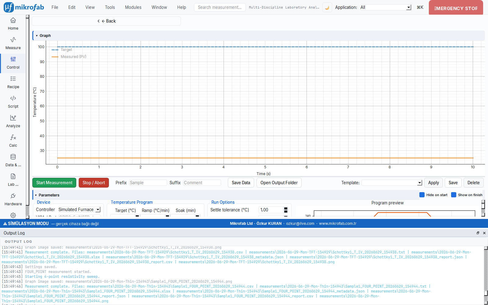
Default program: (100 °C, 5 °C/min, 10 min) → (150 °C, 5 °C/min, 30 min) → (25 °C, 5 °C/min, 0 min). The preview draws the program as a staircase (program_staircase) and shows the estimated total duration.

5.2 Options

Parameter	Unit	Range	Default
Settle tolerance (settle_tol)	°C	0.1 – 50	1.0
Settle timeout (settle_timeout)	min	0.5 – 600	30
Sampling interval	s	0.5 – 600	2.0
Starting temperature (preview)	°C	−100 – 1000	25
Return to ambient (return_ambient)	—	on/off	on
Return temperature	°C	−100 – 1000	25
Hold last value (hold_last)	—	on/off	off

ℹ️

Note If "Return to ambient" is checked, the furnace is brought down to the return_temp value at 5 °C/min when the program ends (safe shutdown).

5.3 Phase Flow and Readout

The engine passes through the following phases in order on each segment: ramp (ramp to target) → soak (hold at target temperature) → once the segments are done, an optional hold and return (return to ambient). The status bar shows the connecting / ramping / soaking / holding / returning / done / aborted tokens, translated.

The readout panel presents a large PV display (°C) + the target (a ✓ mark when settled) + the phase + the segment (seg+1 / total) + the soak countdown (mm:ss). The live plot has two traces: Target (blue dashed) + PV (orange solid), on the time axis; NaN PV (read error) points are skipped.

ℹ️

Note Mock + Save: For SIM (and real types in mock mode), make_furnace_controller(..., mock=True) sets up a simulated furnace; the PV tracks the set-point with a ramp model. Save writes the run's TempProfilePoint rows to CSV.

Common Notes

⛔

Danger Safe state: All instrument-facing paths are protected by timeout + safe-state (output OFF / 0 V) + mock. Stop is a cooperative cancel; on shutdown the worker is told to "stop" and is waited on to finish (the QThread "Destroyed while running" is prevented).

Save: Each module writes the last run to the relevant format with the composite prefix (LCR/RPS → Dataset, Profile/TempProfile/DMM → CSV). On a failed connection the application does not crash; a translated error message is shown in the status bar.
Language/Theme: All panels support EN+TR i18n (tr()) and light/dark theme (apply_theme); user text is not hard-coded.