Photodetector, PV, TFT and Statistical Analyses
This section describes in detail all the core analysis modules in the Analyze workspace. While the Measurement workspace generates data from the instrument, the Analyze workspace extracts physical metrics from a file (CSV) that you load. Each module is a pure core function: analyze_<modul>(dataset, params) -> AnalysisResult. No value that cannot be computed is ever filled with 0; an unknown value is always shown as empty (None, displayed as — in the interface).
examples/analysis/. Each example dataset comes with a hand-derived "ground truth" and is automatically verified by tests/test_realistic_examples.py; that is, the numbers in this manual are bit-for-bit reproducible in the product.
When you take a measurement with an instrument you are left with a pile of numbers (time, current, voltage columns); this section turns that raw table into meaningful physical answers such as "how fast is this photodetector?" or "what is the efficiency of this solar cell?". Just as a blood test analyzer extracts individual values (sugar, iron, cholesterol) from a blood sample, each analysis module computes a specific quantity from the CSV file you load and tells you whether the result is trustworthy.
How it works: Most of the modules in this section interpret the characteristic curve of a device (time response, J-V, transfer, noise spectrum...), because the shape of that curve directly carries the physics within it (exponential rise = RC/trap, J-V series = diode+resistors, sub-threshold line = switching sharpness). Each module extracts the physical parameters from the curve, compares the result against standards (IEC/IEEE/GUM) and against example "ground truth" values, and marks it with a reliability badge. In the module boxes below, the physical meaning, typical range and common interpretation pitfall of each metric are explained one by one.
- Why it is done: a raw signal has no meaning on its own; to make a decision you must convert it into standard, comparable metrics (speed, efficiency, noise, quality).
- What it teaches / measures: dozens of physical quantities for photodetectors, solar cells (PV), thin-film transistors (TFT) and statistics; plus how reliable each result is (the badge).
- Where it is used: device comparison in research labs, quality control in production, result interpretation in classroom/lab experiments, and failure analysis.
1. Common Concepts — Valid Across All Modules
1.1 Role-based automatic column mapping
When you load a CSV, the loader assigns each column a role. The module reads columns by their roles, not by their names; this way files coming from different instruments, with different headers, are "computed automatically" without requiring manual mapping. The main roles:
| Role | Meaning | Typical unit |
|---|---|---|
t | Time / cycle axis | s |
i | Current (main signal) | A |
v | Voltage | V |
i_dark | Dark current (noise series) | A |
p_in | Incident optical power | W |
wavelength | Wavelength | nm |
v_drive | Drive (PWM) signal | V |
v_response | Detector response signal | V |
v_bias | Stepped gate voltage (TFT output family) | V |
Thanks to the match hints in the module's descriptor (e.g. vgs, gate), a file also resolves same-unit ambiguities (e.g. in a TFT output file vgs_set → v_bias step axis, vds_* → v sweep axis). CSV format: comment lines begin with #, followed by a Header [unit] line, then the data; the loader strips the trailing [unit] suffix.
1.2 AnalysisResult — the output envelope of every module
Every module fills the same output structure:
- scalars (results) — named numerical metrics (e.g.
rise_time_s,pce_pct); the unit is carried within the name. - units — the unit of each metric.
- flags — reliability/quality flags (bool), e.g.
metrics_resolved,nep_reliable. - warnings — natural-language warning lines for the user.
- narrative — single-sentence summary.
- plots — plot recipes (time series, log-log, J-V, circuit diagram...).
- note — a line explaining why a value could not be computed when the data is insufficient.
1.3 Reliability badge
A three-state badge is shown above every result. Priority order: unreliable > non_stc > reliable.
| Badge | Meaning | Trigger |
|---|---|---|
| ✓ Reliable reliable | All reliability-determining checks passed | Default |
| ✕ unreliable | Any quality check with sets_reliability=true FAILED | e.g. metrics_resolved False |
| ⚠ Non-STC non_stc (non-standard condition) | A required condition (irradiance / temperature / active_area) was not provided | Provenance condition missing |
Each descriptor also carries diagnostics that, when a check fails, suggest a corrective action to the user (map columns, auto-detect thresholds, open parameters, reload the data, change the axis scale).
1.4 GUM uncertainty framework
Modules that report uncertainty follow the Type-A evaluation of ISO/IEC Guide 98-3:2008 (GUM):
sample standard deviation   s = sqrt( Σ(x_i - x̄)² / (N-1) )      (Bessel correction)
uncertainty of the mean     u(x̄) = s / sqrt(N)                  (Type-A)
expanded uncertainty        U = k · u(x̄)                        (k = coverage factor, default 2)
The single formatter in the interface, format_quantity, writes the ± term only when u_std > 0 AND n ≥ 2; if a value is missing it shows an em dash —, never 0. Numbers are shown with SI prefixes (n, µ, m, k, M...); %, dB, Jones and composite units take no prefix.
2. Photodetector Analysis Modules
2.1 Temporal Response — temporal_response (Module 1)
When you suddenly switch the light on and off at a light detector, its output does not jump instantly; it rises and decays with some delay. This module turns the question "how quickly does it respond?" into a number. Just like measuring how many seconds a car takes to go from 0 to 100 km/h — it shows how fast the detector reaches the light and how fast it stops.
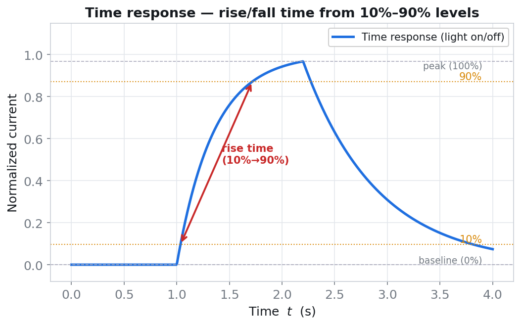
Physical background: When the light turns on, photons are absorbed and carriers are generated, but those carriers accumulate charge in the device capacitance (and load resistance); the system behaves like an RC circuit and carries the output to its saturation level not instantaneously but exponentially. That is why the time series is not a sharp step but a smooth "rising-exponential / decaying-exponential" shape; the 10%→90% transition takes exactly ln(9)·τ ≈ 2.197·τ in a single-pole system. When the light turns off the same RC discharges; if the material contains traps, the fall/recovery is noticeably slower than the rise (asymmetry = trapping fingerprint).
- Why it is done: to understand whether the detector can follow fast signals (e.g. high-speed communication, pulsed light) without distorting/missing them.
- What it teaches / measures:
rise_time_s= the time for the output to climb from 10% to 90% when the light turns on (turn-on speed);fall_time_s= the time to drop from 90% to 10% when the light turns off (turn-off speed);recovery_time_s= the time to return to the baseline (baseline+5%), capturing persistent effects; thet_fall/t_riseratio indicates symmetry (≈1 clean, ≫1 trapping);n_cyclesis the number of on/off cycles averaged. - Typical values and interpretation: fast Si PIN photodiodes ns–µs; phototransistors µs; a-Si / organic / perovskite photoconductors are considered "slow" at the ms–s scale.
t_fall ≈ t_riseis ideal; ift_fallis much larger, there are deep traps / persistent photoconductivity. - Common mistake / caution: if sampling is too sparse (Nyquist: if
t_r ≥ 1/f_sis not satisfied) the rise time is measured larger than it is — check thenyquist_okflag. On a noisy signal the baseline/peak may be misestimated and the thresholds may shift; if no transition is found, review the threshold percentages. - Where it is used: optical communication receiver selection, sensor design validation, fast photo-switch characterization, and trap/persistence diagnosis in materials.
What it does: Extracts the rise, fall and recovery times from a photo-switching (light on/off) time series.
Columns (roles): Required: t, i. Optional: v (voltage data + can be converted to current via r_load_ohm).
| Parameter | Unit | Description | Default |
|---|---|---|---|
threshold_low_pct | % | Low threshold (start of rise) | 10.0 |
threshold_high_pct | % | High threshold (end of rise) | 90.0 |
recovery_pct | % | Recovery threshold (baseline+%) | 5.0 |
r_load_ohm | Ω | Load resistance (for V→I conversion) | 0.0 |
Applied formula: Baseline (dark) = mean of the lowest 10%; peak = mean of the highest 5%; amplitude amp = peak − dark. Levels are dark + {10, 90, 5}% × amp. For each cycle t_rise = t(90%) − t(10%), and the mean is taken. Closed form in a single-pole RC system:
Outputs: rise_time_s, rise_time_std_s, fall_time_s, fall_time_std_s, recovery_time_s [s]; dark_level, peak_level [A]; n_cycles.
Reliability / quality flags: rise_time_reliable — Nyquist check (t_r ≥ 1/f_s). Descriptor checks: cycles_found (n_cycles ≥ 1, determines reliability), above_floor (signal_range > 3·noise_sigma, determines reliability), nyquist_ok (warning). Standards: IEEE 181-2011, IEC 60469:2013, GUM.
Example data / expected result: examples/analysis/01_temporal_response.csv (single-pole RC, 3 cycles, τ_r=20 µs, τ_f=60 µs). Expected: t_rise = 43.944 µs, t_fall = 131.833 µs, t_fall/t_rise = 3.0, n_cycles = 3.
note is populated), review the threshold percentages or the baseline level; on a very noisy signal, raising threshold_low_pct improves stability.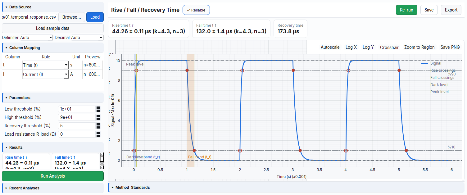
temporal_response module — extracting rise/fall/recovery from a photo-switching time series.A single on/off cycle in the time series is used; the amplitude is found from the baseline (dark) and peak levels, and the horizontal 10% and 90% level lines are marked.
- First the baseline (mean of the lowest 10%) and the peak (mean of the highest 5%) are determined; with amplitude
amp = peak − darkthe10%and90%levels are drawn. - The time values at which the rising edge crosses these two levels are read (with linear interpolation between neighboring points if needed); the same is done from 90%→10% for the fall.
- Result:
t_rise = t(90%) − t(10%),t_fall = t(10%) − t(90%)and the cycles are averaged; in a single-pole RC,t_rise = ln(9)·τ ≈ 2.197·τ.
2.2 Photo/Dark Current Ratio — photo_dark_ratio (Module 2)
A light detector produces a small "dark current" even when there is no light; when light arrives the current grows much larger. This module computes the ratio of the two and how clearly the signal is distinguished relative to the noise (SNR). Like being able to hear a whisper in a quiet room — the lower the ambient noise, the more confidently you can pick out the real signal.
Physical background: Dark current arises from thermally generated carriers without light and from leakage (generation-recombination, surface leakage, reverse-bias leakage); this is the detector's "baseline". When light arrives, photo-generated carriers ride on top of it and carry the current upward, so in the time series you see two stable plateaus (dark and light); the height of the jump in between is I_photo. The small fluctuation on the dark plateau is the noise (σ); whether you can confidently read the signal as "on/off" depends on how many times this jump exceeds the noise.
- Why it is done: to measure whether the detector can distinguish weak light from the background (dark current + noise) and how "clean" an on/off contrast it provides.
- What it teaches / measures:
i_dark= lightless baseline current (the smaller the better);i_photo= the net current increase with light;photo_dark_ratio = I_photo/I_dark= contrast (large = good);noise_sigma= standard deviation of the dark region;snr_db = 20·log10(|I_photo|/σ)= how many dB the signal is above the noise. - Typical values and interpretation: for a good photodiode a ratio of 10³–10⁶ and SNR of tens of dB (e.g. ~60 dB is very clean) is expected; if the ratio is <10 the signal is drowned in the background. Dark current rises exponentially with temperature, so low
I_dark= low noise and the ability to see weaker light. - Common mistake / caution: reading SNR linearly instead of in log (dB) and misinterpreting it; not measuring the dark plateau long enough (σ is poorly estimated); if the light region hits saturation/compliance,
I_photocomes out smaller than it is. The ratio and SNR are different: one measures contrast, the other distinguishability relative to noise. - Where it is used: low-light-level detection, sensor quality control, material comparison, and temperature-dependent dark-current diagnosis.
What it does: Computes the photo/dark current ratio and the signal-to-noise ratio (SNR) from a square optical step.
Columns: Required: i. Optional: t. No parameters.
Applied formula: The stable dark (below baseline+10%) and light (above baseline+90%) regions are separated; noise σ = std(dark region).
I_photo = I_light − I_dark
ratio   = I_photo / I_dark
SNR[dB] = 20 · log10( |I_photo| / σ )
Outputs: i_dark, i_photo, noise_sigma [A]; photo_dark_ratio (dimensionless); snr_db [dB]. Flag: dark_current_resolved.
Example / expected: 02_photo_dark_ratio.csv (I_dark=100 nA, I_light=10 µA, σ=10 nA). Expected: ratio = 99.0, SNR = 20·log10(990) = 59.91 dB.
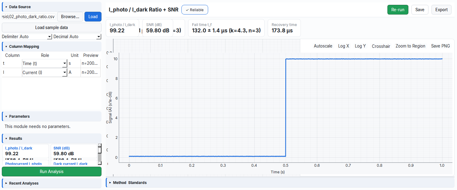
photo_dark_ratio module — photo/dark current ratio and SNR in dB.2.3 Persistence / Trapping — persistence (Module 3)
When you turn the light off, the signal of some detectors does not reset immediately but stays "stuck" for a while; this is because traps in the material release the charge carriers late. This module models that slow decay and extracts how long it lasts. Like a glow-in-the-dark toy that keeps glowing for a while after the light is switched off.
Physical background: Some of the carriers generated under light are captured at defect/trap levels; when the light turns off these traps release the charge thermally late, so the current does not drop to zero instantly (persistent photoconductivity, PPC). If there is a single trap depth the decay is single-exponential (exp(−t/τ)); if the traps are distributed the curve bends into a "stretched exponential" (stretched, β<1) or a double-exponential with two separate time scales. That is why it is typical to see a fast initial drop followed by an extended tail; the module turns the character of this tail into a number by selecting the model with the highest R².
- Why it is done: to understand the defect/trap density in the material and whether the device exhibits a "memory effect" (slow reset).
- What it teaches / measures:
persistence_tau_s= the characteristic time constant τ of the decay (large = long memory/deep trap);persistence_model= the selected model (single/stretched/double);persistence_beta= the stretching exponent β (close to 1 = single time scale, <1 = wide trap distribution);persistence_r2= how well the model fits the data. - Typical values and interpretation: τ µs–ms in fast crystalline detectors; τ can be seconds–minutes in trap-heavy a-Si/oxide/perovskite/organic devices. β≈1 clean single-trap; β≈0.3–0.7 distributed traps; if R²<0.95 a single model is insufficient and the module suggests an alternative.
- Common mistake / caution: a wrong detection of the light-off instant ruins the entire fit; if the window is chosen too short the long tail is not seen and τ comes out small. Forcing a single-exponential misreports the physics of a double-exponential decay — read R² and the model selection together.
- Where it is used: new-material research, defect/trap diagnosis, suitability assessment for applications requiring fast repetition (high frame-rate imaging, etc.).
What it does: Fits the slow decay of the signal after the light is turned off (persistent photoconductivity / trapping) with exponential models and extracts the time constant.
Columns: Required: t, i. No parameters.
Applied formula: The light-off instant is detected, the subsequent region is isolated, and three candidate models are fitted; the model with the highest R² is selected:
- Single exponential:
I = A·exp(−(t−t₀)/τ) + C - Stretched:
I = A·exp(−((t−t₀)/τ)^β) + C - Double exponential:
I = A₁·exp(−t/τ₁) + A₂·exp(−t/τ₂) + C
Outputs: persistence_model, persistence_r2, persistence_tau_s [s], persistence_beta, single_exp_tau_s, single_exp_r2. Warning: an alternative model is suggested if R² < 0.95.
Example / expected: 03_persistence_decay.csv (single exponential, τ=0.25 s). Expected: single_exp_tau_s ≈ 0.25 s, R² ≈ 1.0.
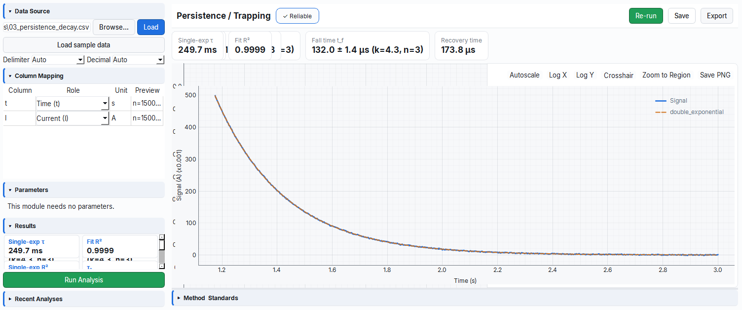
persistence module — decay time constant with exponential/stretched/double-exponential model selection.2.4 -3 dB Bandwidth — bandwidth_3db (Module 8)
It converts how fast a detector responds (rise time) directly into the answer to "what is the highest-frequency signal it can follow, in Hz?". Like computing how many steps per minute a runner can take from their stride speed — speed and frequency are two faces of the same coin.
Physical background: A system that is "slow" in the time domain is "narrow-band" in the frequency domain; the same RC/single-pole behavior locks these two faces together. For a single-pole low-pass there is a fixed relation between the corner frequency at which the gain falls to -3 dB (half the power) and the 10%–90% rise time: BW·t_r ≈ 0.35. That is, you can invert the measured rise time to estimate the highest frequency that the device can pass with less than 30% attenuation; this is why you read the speed limit without performing a separate frequency sweep.
- Why it is done: to know whether the detector can pass a signal (modulation, pulse train) at a given frequency without attenuation, without performing a separate frequency sweep.
- What it teaches / measures:
rise_time_s= the 10%–90% rise time used (fromtemporal_responseif not provided);bandwidth_3db_hz= the -3 dB bandwidth derived from it (large = fast device). RelationBW = 0.35/t_r. - Typical values and interpretation: ms rise → kHz band; µs → hundreds of kHz–MHz; ns → GHz scale. The 0.35 coefficient is a single-pole/Gaussian approximation; in multi-pole or trap-dominated devices the real bandwidth may deviate, and the result should be read as an order-of-magnitude estimate.
- Common mistake / caution: if the rise time was measured with sparse sampling that violates Nyquist, the derived bandwidth is also wrong; also, if the fall time is much larger than the rise time (trapping), the bandwidth derived from a single
t_roverstates the true repetition rate. - Where it is used: high-speed optical link design, sensor specification validation, and speed-limit (modulation band) estimation.
What it does: Derives the -3 dB bandwidth from the rise time (Gaussian/single-pole approximation).
Columns: Optional: t, i. Parameter: rise_time_s (if 0, computed from the data via temporal_response).
Outputs: rise_time_s [s], bandwidth_3db_hz [Hz].
Example / expected: 04_bandwidth_3db.csv (the same RC pulse). t_rise = 43.944 µs → BW = 0.35 / 43.944 µs = 7964.9 Hz.
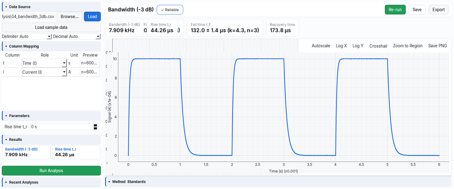
bandwidth_3db module — deriving the -3 dB bandwidth from the rise time.No separate frequency-sweep plot is needed; the 10%–90% rise time read from temporal_response (see 2.1) is inverted.
- The rise time
t_ris taken (by reading the 10%–90% levels from the time series). - Result:
BW = 0.35 / t_r(single-pole/Gaussian approximation); e.g.t_r = 43.944 µs → BW ≈ 7965 Hz.
2.5 Spectral Responsivity — responsivity (Module 4)
It tells you how much current the detector produces for each watt of light falling on it — that is, the device's "sensitivity to light". Like how much electricity a solar panel produces under the same sun; a detector that produces more current under the same light is more responsive.
Physical background: Each absorbed photon produces at most one electron-hole pair (in the absence of gain), so the current is directly proportional to the optical power and the slope gives the responsivity (R = I_photo/P). Since the energy of a photon is E = hc/λ, at constant power there are more photons at long wavelengths; therefore R tends to increase linearly with λ even if the quantum efficiency stays constant (R = EQE·qλ/hc) until the material's band gap is exceeded and absorption drops. This is why the R(λ) curve peaks and then falls: surface loss at short λ, band-gap cutoff at long λ.
- Why it is done: to compare the efficiency of different detectors under the same light, to calibrate the measurement chain, and to find which color it is most sensitive to.
- What it teaches / measures:
responsivity_a_w= responsivity in A/W (the slope);i_photo= net photocurrent;p_detector_w= the power that actually falls on the detector, with active/spot area scaling; in spectral moderesponsivity_peak_a_wandpeak_wavelength_nm= the peak of R(λ) and its wavelength. The implied EQE = R·1239.84/λ also shows the per-photon yield. - Typical values and interpretation: for a Si photodiode R ~0.3–0.6 A/W in the visible–near IR (peak ~0.6 at ~900 nm); for InGaAs ~0.8–1.0 A/W (1550 nm). R exceeding the
qλ/hclimit (EQE=1) is only possible with internal gain (APD, phototransistor); otherwise it indicates a measurement/power error. - Common mistake / caution: the most critical input is the incident power
p_in_w; a wrong/uncalibrated power scales the entire R. If the spot area is larger than the active area, part of the light does not fall on the detector — if area scaling is not entered, R comes out smaller than it is. If you see EQE>100% (and gain is not expected), first check the power and area. - Where it is used: detector selection, spectral characterization, calibration, and production quality control.
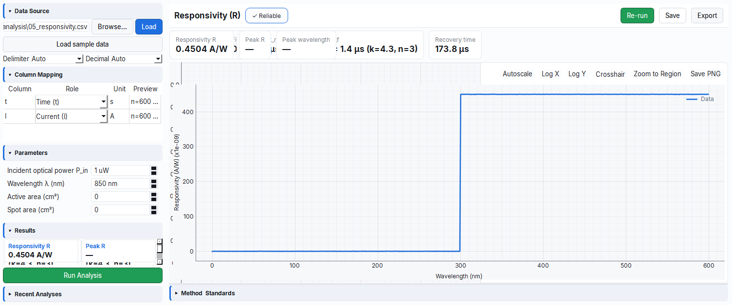
What it does: Computes responsivity from photocurrent / incident optical power; if a wavelength table is present it extracts the R(λ) curve.
Columns: Required: i. Optional: t, wavelength.
| Parameter | Unit | Description | Default |
|---|---|---|---|
p_in_w | W | Incident optical power (REQUIRED) | 1e-6 |
wavelength_nm | nm | Wavelength | 850.0 |
active_area_cm2 | cm² | Active area | 0.0 |
spot_area_cm2 | cm² | Spot area | 0.0 |
Applied formula: The power falling on the detector is P_det = P_in·(A_active/A_spot) (if the spot is larger than the active area), otherwise P_det = P_in. Then:
R = I_photo / P_det            [A/W]
implied EQE = R · 1239.84 / λ    (≤ 1, if no gain)
Outputs: i_photo [A], p_detector_w [W], responsivity_a_w [A/W]; in spectral mode responsivity_peak_a_w, peak_wavelength_nm. Standard: IEC 60904-8.
Example / expected: 05_responsivity.csv (Si photodiode, 850 nm, P_in=1 µW). I_photo = 0.45·1 µW = 450 nA → R = 0.45 A/W, implied EQE = 65.6%.
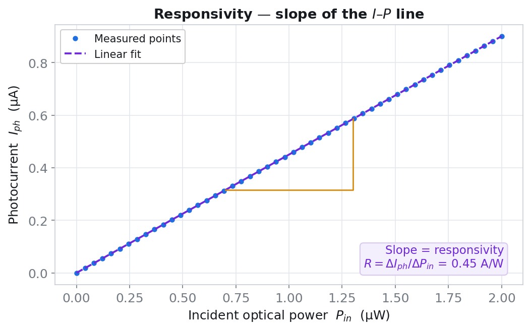
responsivity module — responsivity in A/W and the R(λ) spectral curve when needed.The net photocurrent I_photo is plotted against the power falling on the detector P_det; the slope of the line directly gives the responsivity (A/W).
- If there are multiple power points, a line through the origin is fitted to the
I_photo–P_detpoints. - The slope of the line is taken (if there is a single point,
R = I_photo/P_detis found from a single ratio). - Result:
R = ΔI_photo/ΔP_det[A/W]; from this the impliedEQE = R·1239.84/λis derived.
2.6 Quantum Efficiency — eqe_iqe (Module 5)
It tells you, as a percentage, how many out of every 100 light particles (photons) striking the device are converted into electric charge. Like inviting 100 guests and counting how many came in — EQE is based on all the photons that strike, while IQE accounts for those that turn back at the door (reflected light) to give the "true" fraction of those that came in.
Physical background: While responsivity ties the current to watts, quantum efficiency normalizes the count per photon: since a photon's energy is hc/λ, EQE = R·(hc/qλ) = R·1239.84/λ[nm]. EQE includes all losses — reflected + unabsorbed + recombined — so it can understate the true collected-charge efficiency. IQE is based only on the photons that enter (are absorbed): IQE = EQE/(1−R_refl). Therefore IQE is always greater than (or equal to) EQE and tells you "how well the material collects what it absorbs, reflection aside".
- Why it is done: to see how hard the device pushes the fundamental limit of converting light into load (each photon → one charge) and to separate whether the loss is from reflection or from collection/recombination.
- What it teaches / measures:
eqe_pct= the percentage of charge collected per incident photon (external);iqe_pct= the efficiency per absorbed photon after reflection is removed (internal);responsivity_a_wandwavelength_nm= the inputs of the calculation. Theeqe_needs_reflection_correctionflag indicates that reflection data is required for IQE. - Typical values and interpretation: for a good Si detector/cell, peak EQE can be 80%–95% and IQE >90%; an anti-reflection coating brings EQE closer to IQE. EQE or IQE exceeding 100% (with no gain mechanism) is suspicious and the module issues a warning.
- Common mistake / caution: entering a wrong λ scales EQE directly (the formula is inversely proportional to λ); mistaking IQE for "internal efficiency" without entering reflection (
R_refl); mistaking EQE>100% for gain when it is usually a power/area/λ error. - Where it is used: solar cell/detector research, material and anti-reflection coating optimization, efficiency comparison.
What it does: Computes external (EQE) and internal (IQE) quantum efficiency.
Columns: No required column. Optional: i, t.
| Parameter | Unit | Description | Default |
|---|---|---|---|
wavelength_nm | nm | Wavelength (REQUIRED) | 850.0 |
responsivity_a_w | A/W | R (from data if not provided) | 0.0 |
reflectance | — | Reflectance R_refl | 0.0 |
p_in_w | W | Incident power (for R) | 0.0 |
active_area_cm2 / spot_area_cm2 | cm² | Area scaling | 0.0 |
Applied formula:
EQE = R · hc/(q·λ) = R · 1239.84 / λ[nm]      (0..1)
IQE = EQE / (1 − R_refl)
If R is not provided, it is derived from the data via R = I_photo/P_det.
Outputs: responsivity_a_w, wavelength_nm, eqe_pct [%], iqe_pct [%]. Flag: eqe_needs_reflection_correction. Warning: if EQE or IQE > 100% (suspicious if there is no gain mechanism).
Example / expected: 06_eqe_iqe.csv (R=0.45 A/W, λ=850 nm, R_refl=10%). EQE = 65.64%, IQE = 65.64/0.9 = 72.94%.
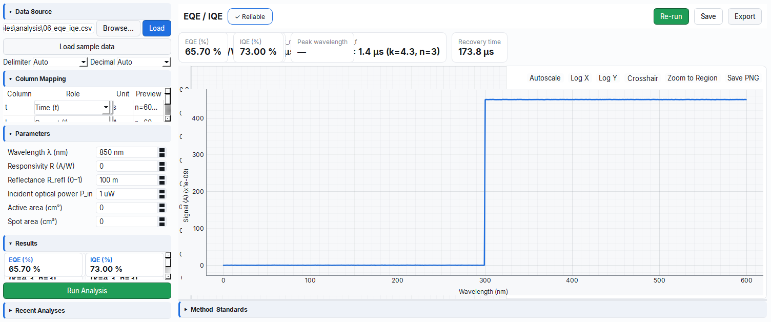
eqe_iqe module — computing EQE/IQE from responsivity and wavelength.No slope/tangent is taken from a plot; it is computed directly by formula from the responsivity R and the wavelength λ.
- The responsivity
R(A/W) is taken (from the data viaR = I_photo/P_detif not provided). - Result:
EQE = R·1239.84/λ[nm](0..1); with reflection correctionIQE = EQE/(1 − R_refl).
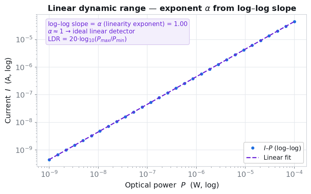
2.7 Linearity and LDR — linearity_ldr (Module 6)
When you double the light, does the current double too? This module measures how "honestly proportional" the detector is to the incident power and over what brightness range it stays reliable. Like a scale being able to weigh both one gram and one kilogram accurately — proportionality must not break over a wide range.
Physical background: In an ideal detector the photocurrent is one-to-one proportional to the incident power (I ∝ P¹), because twice the photons produce twice the carriers. In reality the proportionality breaks when traps saturate at low power or recombination increases at high power; the relationship is summarized by the power law I = C·P^α, which becomes a straight line on a log-log plot with slope α. α=1 is perfectly linear; α<1 (sub-linear) charge trapping/recombination; α>1 (super-linear) indicates a gain mechanism. The span between the smallest and largest power over which the device preserves proportionality is the linear dynamic range (LDR).
- Why it is done: to find over what light range the detector's measurement can be trusted and where it enters saturation/trapping/gain.
- What it teaches / measures:
linearity_alpha= the power-law exponent α (regime indicator);powerlaw_coeff= the coefficient C (scale);linearity_r2= the quality of the log-log fit;ldr_db = 20·log10(P_max/P_min)= the linear dynamic range;p_min_w/p_max_w= the ends of the range. - Typical values and interpretation: in a good detector 0.95 ≤ α ≤ 1.05 and LDR is tens–100+ dB (several decades); values like α=0.5 indicate a strong trapping regime. If R²<0.999, the whole range does not obey a single linear law (curvature at the ends).
- Common mistake / caution: assessing linearity "by eye" on a normal (linear) axis — it must be viewed log-log; claiming a wide LDR with only a few points; mistaking the detector saturating at the brightest point and lowering α for a material defect. LDR is converted to dB with 20·log10, not with the number of decades (1 decade = 20 dB).
- Where it is used: measurement instrument calibration, sensor operating-range definition, and detection of gain/trapping behavior.
What it does: Extracts the power-law dependence of the photocurrent on the incident power and the linear dynamic range (LDR).
Columns: Required: p_in, i. No parameters.
Applied formula: Log-log power-law fit I = C · P^α; then:
Regime classification: 0.95 ≤ α ≤ 1.05 linear; α < 0.95 sub-linear (trapping); α > 1.05 super-linear (gain).
Outputs: linearity_alpha, powerlaw_coeff (C), linearity_r2, ldr_db [dB], p_min_w, p_max_w [W]. Warning: if R² < 0.999 the full range is not linear. Standard: IEC 60904-10.
Example / expected: 07_linearity_ldr.csv (5 decades, α=1). α = 1.0, LDR = 20·log10(1e5) = 100 dB, C = 0.45.
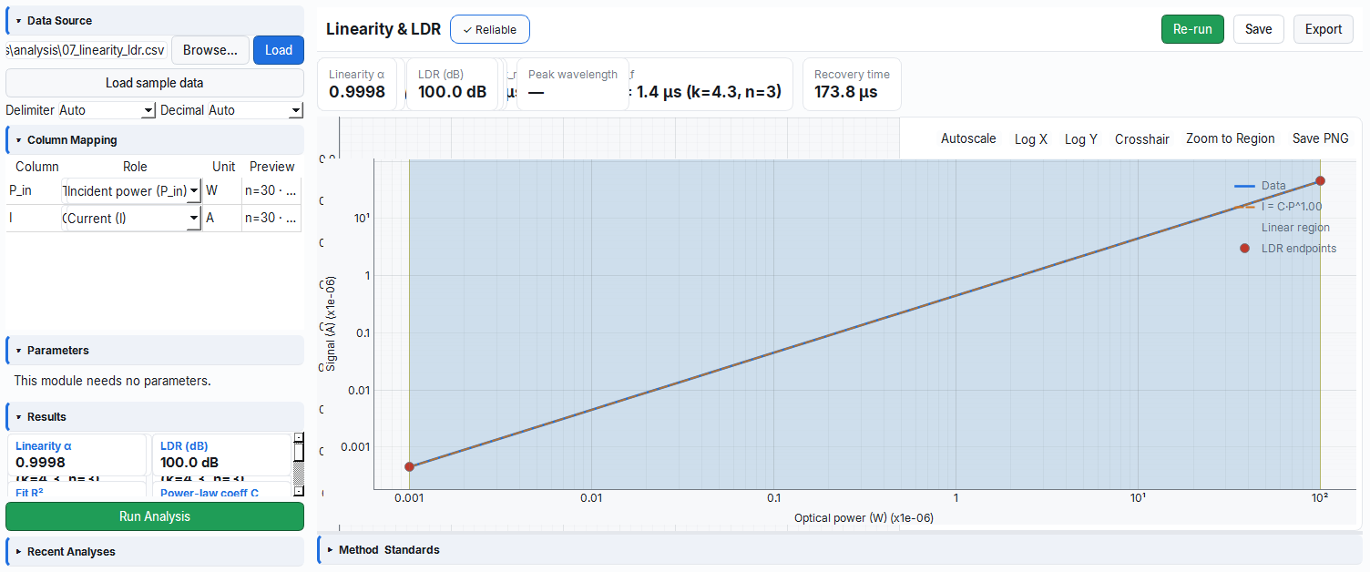
linearity_ldr module — log-log power-law fit and LDR in dB.The I–P data is plotted on log–log axes; the power law I = C·P^α becomes a straight line here.
- A line is fitted to the log–log points (
log Iversuslog P). - The slope of the line gives the exponent:
α = Δ(log I)/Δ(log P); the coefficientCis read from the intercept. - Result: from the ends where linearity is preserved,
LDR[dB] = 20·log10(P_max/P_min);0.95 ≤ α ≤ 1.05is accepted as linear.
2.8 NEP and Detectivity — nep_detectivity (Module 7)
What is the "weakest light" a detector can detect? This module measures the device's own noise and computes the light power that produces a signal equal to that noise (NEP) and a size-independent quality figure (D*). Like determining the faintest sound you can hear in a noisy environment — the quieter the device, the weaker the signal it can catch.
Physical background: There is always random current fluctuation at the baseline of a detector (shot noise from the dark current √(2qIΔf) and Johnson/thermal noise from the shunt resistance √(4k_BTΔf/R)). You have "seen" a signal only when you can lift it above this noise floor; the optical power that produces a current equal to the noise is the noise-equivalent power (NEP = i_noise/R). Since a larger area or wider band collects more noise, the specific detectivity D* = R·√(A·Δf)/i_noise is defined to normalize these for fair comparison of devices — the larger D*, the more sensitive the device.
- Why it is done: to determine the detector's sensitivity limit (the weakest detectable light) and to fairly compare devices of different size/band/technology.
- What it teaches / measures:
nep_w_sqrthz= band-normalized noise-equivalent power (small = sensitive);nep_total_w= total NEP over the whole band;detectivity_jones= area/band-normalized D* (large = good);noise_density_a_sqrthz= current noise density;shot_noise_a/thermal_noise_aandnoise_dominant= which noise mechanism dominates. - Typical values and interpretation: for room-temperature Si/InGaAs D* ~10¹¹–10¹³ Jones is realistic; cooled IR detectors are on the order of 10¹⁰–10¹². D*>10¹⁴ Jones (with no gain) is physically suspicious and the module issues a warning; the smaller the NEP, the weaker the light the device can pick out.
- Common mistake / caution: R (responsivity) is a REQUIRED input; a wrong R scales NEP and D* directly. If the bandwidth Δf and area A are not entered, the comparison becomes meaningless. NEP (W/√Hz) must not be confused with NEP_total (W); very small D* values are preserved with significant-figure rounding (decimal rounding would have shown 0).
- Where it is used: low-light/infrared detector selection, performance ranking, and noise-source (shot vs thermal) diagnosis.
What it does: Computes the noise-equivalent power (NEP) and the specific detectivity (D*) from a dark-current noise series.
Columns: Required: i_dark. Optional: t, i.
| Parameter | Unit | Description | Default |
|---|---|---|---|
responsivity_a_w | A/W | R (REQUIRED) | 1.0 |
active_area_cm2 | cm² | Active area | 0.01 |
bandwidth_hz | Hz | Measurement bandwidth Δf | 1.0 |
temperature_k | K | Temperature | 300.0 |
shunt_resistance_ohm | Ω | Shunt resistance (thermal noise) | 0.0 |
Applied formula: σ = std(I_dark); band-scaled RMS current:
i_noise        = σ · sqrt( Δf / (f_s/2) )
noise_density  = i_noise / sqrt(Δf)          [A/√Hz]
NEP            = noise_density / R            [W/√Hz]
NEP_total      = i_noise / R                  [W]
D*             = R · sqrt(A·Δf) / i_noise     [Jones]
i_shot         = sqrt( 2·q·|I_dark| · Δf )
i_thermal      = sqrt( 4·k_B·T·Δf / R_shunt )
Dominant noise: if i_shot ≥ i_thermal then shot, otherwise thermal.
Outputs: i_dark_mean, i_noise_a, noise_density_a_sqrthz, nep_w_sqrthz, nep_total_w, detectivity_jones [Jones], bandwidth_hz, shot_noise_a, thermal_noise_a, noise_dominant. Flag: nep_reliable. Warning: D* > 1e14 Jones (suspicious for Si/InGaAs). Standard: GUM. Very small values are preserved with significant-figure rounding (decimal rounding would have reduced them to 0).
Example / expected: 08_nep_detectivity.csv (I_dark mean 1 nA, σ≈1 pA, f_s=1 kHz, R=0.45 A/W, A=0.01 cm², Δf=1 Hz). D* ≈ 1e12 Jones (realistic Si).
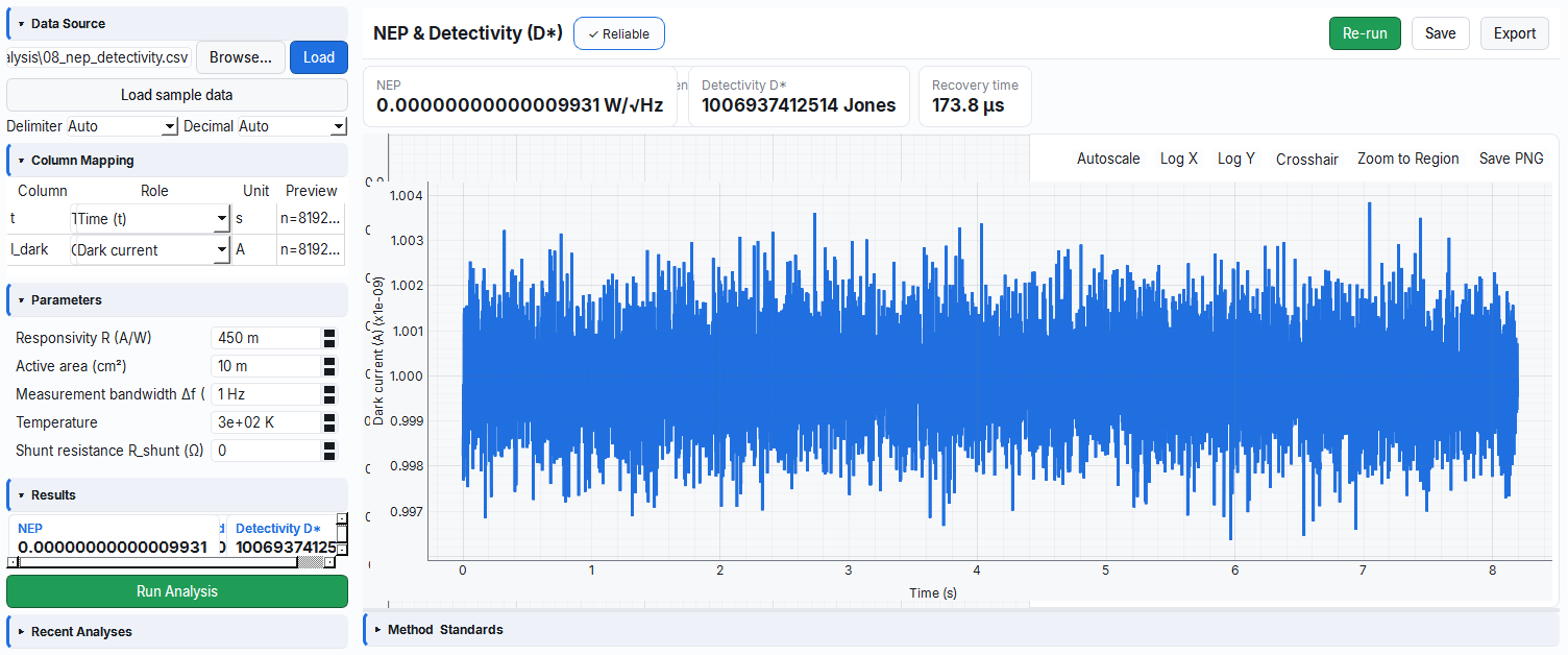
nep_detectivity module — noise-equivalent power and detectivity in Jones.No slope is taken from a plot; the standard deviation σ of the dark-current series is measured and scaled by the responsivity R.
- The noise of the dark region
σ = std(I_dark)and the band-scaled RMS currenti_noiseare computed. - Result:
NEP = (i_noise/√Δf)/R[W/√Hz];D* = R·√(A·Δf)/i_noise[Jones].
2.9 Noise PSD — noise_psd (Module 9)
Every device has noise, but this noise is not uniform; it comes from different sources at different frequencies. This module breaks the noise down by frequency and tells you which mechanism dominates (1/f flicker, shot, thermal). Like listening to the hum of an orchestra and separating "is this coming more from the bass drum or the violins?".
Physical background: When you transform the dark-current time series into frequency (PSD), different noise mechanisms leave different signatures. Shot and thermal noise give a flat "white" floor at all frequencies (frequency-independent); in contrast, flicker noise arising from the trap capture-release dynamics is large at low frequency and decreases with frequency as 1/f^γ. That is why on a log-log PSD plot you see a sloped (1/f) region at low frequency and a flat floor at high frequency; the "corner frequency" where the two cross is the point at which flicker submerges into the white floor. Operating above the corner minimizes the noise.
- Why it is done: to find the root cause of the noise (trap-dominated, or fundamental shot/thermal) so the right improvement can be made (filtering, choice of operating frequency, material/process).
- What it teaches / measures:
flicker_gamma= the low-f slope γ (close to 1 means classic 1/f);corner_freq_hz= the corner frequency where flicker drops to the white floor;white_floor_a2_hz= the white noise floor;shot_level_a2_hz/thermal_level_a2_hz= the theoretical shot/thermal levels;low_freq_fit_r2andnoise_dominant= fit quality and the dominant mechanism. - Typical values and interpretation: γ≈1 pure 1/f flicker (trap/defect dominated); γ≈0 white (shot/thermal dominated). A low corner frequency = clean, low-trap material; a high corner = defect-heavy device where operating at low frequencies is difficult. The measured white floor being close to the theoretical shot level indicates the device has reached the fundamental limit.
- Common mistake / caution: if the sampling frequency (
sampling_hz) is wrong the entire frequency axis shifts; a too-short series cannot resolve low frequencies (the corner is not seen). Reading the PSD on a linear axis hides the 1/f region; interpret γ not on its own but together with the corner frequency and the fit R². - Where it is used: low-noise detector/circuit design, material/process quality diagnosis, and operating-band optimization.
What it does: Computes the power spectral density (PSD) of the dark-current series; separates the 1/f^γ flicker, shot and thermal mechanisms.
Columns: Required: i_dark. Optional: t, i. Parameters: sampling_hz (from the time axis if 0), temperature_k=300, shunt_resistance_ohm=0.
Applied formula: PSD from the periodogram; in the low-f region (first 40%) a log-log linear fit gives the slope; γ = −slope. White floor = median of the upper 30%. The corner frequency is where the fit line crosses the white floor:
shot_level    = 2·q·|I_mean|          [A²/Hz]
thermal_level = 4·k_B·T / R_shunt      [A²/Hz]
Dominant: if γ > 0.5 then flicker (1/f), otherwise shot/thermal.
Outputs: flicker_gamma, low_freq_fit_r2, white_floor_a2_hz, corner_freq_hz [Hz], shot_level_a2_hz, thermal_level_a2_hz, noise_dominant.
Example / expected: 09_noise_psd.csv (target PSD S(f) = S_w·max(f_c/f, 1), S_w=1e-22 A²/Hz, f_c=200 Hz). γ = 1.0, floor = 1e-22, corner = 200 Hz, dominant = "flicker (1/f)".
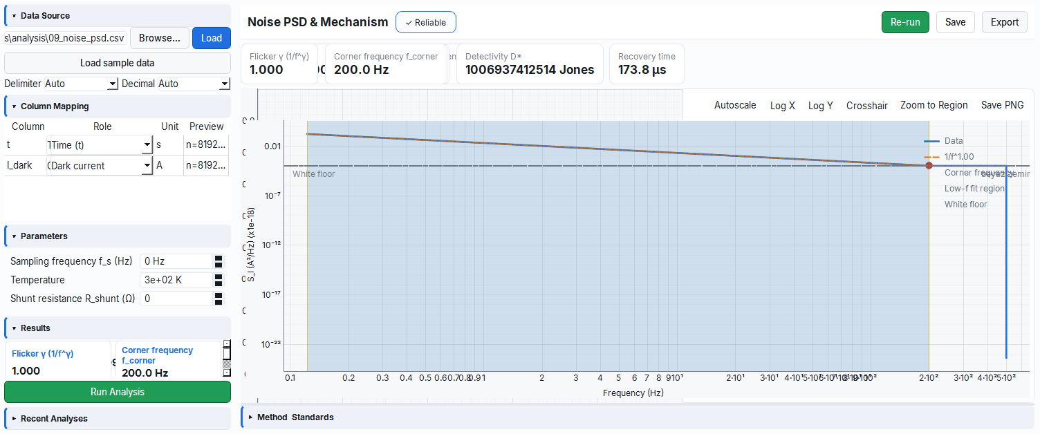
noise_psd module — separating the 1/f flicker, shot and thermal noise mechanisms.The PSD is plotted on log–log axes; a line is fitted to the low-frequency (first 40%) region and the slope is taken.
- A line is fitted to the low-f points (
log Sversuslog f); the negative of the slope gives the exponent:γ = −slope. - Result: the point where the white floor (median of the upper 30%) crosses the fit line is the corner frequency.
2.10 PWM Drive Analysis — pwm_analysis (Module 10)
Light sources such as LEDs are often driven with a very fast on-off (PWM) signal; the frequency of this flicker invisible to the eye, how much of it is "on" (duty cycle) and how clean it is all matter. This module measures the drive signal and, if a detector response is present, finds the delay between them. Like reading the rate and rhythm of a heart with an ECG.
Physical background: In PWM the average brightness is proportional to how much of a constant-amplitude pulse is "on" (the duty cycle); the eye perceives this as continuous light, but the signal is actually a square wave. The module extracts the frequency from the time between rising edges, the duty from the on-fraction, and the ripple from the peak-to-peak variation at the on level; an ideal square wave consists of a fundamental frequency and its harmonics in the FFT, and as distortion increases (sloped edges, ringing) the harmonic content (THD) grows. If a detector response is also present, the time shift between drive and response gives the system's response delay/phase.
- Why it is done: to verify that the drive signal is at the correct frequency/brightness and undistorted, and to measure the drive→detector system delay.
- What it teaches / measures:
frequency_hz(±frequency_std_hzstability) = the pulse frequency;duty_cycle= the on-fraction (average brightness);ripple_pp= the peak-to-peak ripple at the on level;thd= harmonic distortion (the "cleanliness" of the signal);v_high/v_low= the levels; if a response is presentresponse_delay_s/response_phase_deg= delay/phase. - Typical values and interpretation: for flicker-free visible lighting a frequency ≳ a few hundred Hz–kHz is preferred; the duty maps to the desired brightness (e.g. 30% = dim); low ripple and low THD mean a clean drive. A large
frequency_stdmeans an unstable drive (jitter). - Common mistake / caution: if the thresholds (
v_high/v_low) are auto-detected incorrectly on a noisy signal the duty/frequency shifts; if the sampling is too sparse relative to the pulse width the duty and THD become unreliable. When measuring the response delay, the drive and response must be on the same time axis. - Where it is used: LED driver verification, optical-system timing, and control-electronics quality control.
What it does: Extracts frequency, duty cycle, ripple and THD from a drive (PWM) signal; if a detector response signal is present, performs a delay/phase correlation.
Columns: Required: t, v_drive. Optional: v_response, i_drive. Parameters: v_high, v_low (if 0, auto from the 95th/5th percentile respectively).
Applied formula: Threshold 0.5·(V_high+V_low); frequency from the period between rising edges f = 1/⟨T⟩; for each period duty = t_on/T; ripple = peak-to-peak of the high level; THD from the FFT fundamental and harmonics.
Outputs: frequency_hz, frequency_std_hz, duty_cycle, ripple_pp, thd, n_periods, v_high, v_low; response_delay_s, response_phase_deg (if a response is present).
Example / expected: 10_pwm_analysis.csv (ideal square wave, 10 periods). f = 1000 Hz, duty = 30%, V_high = 5 V, V_low = 0 V.
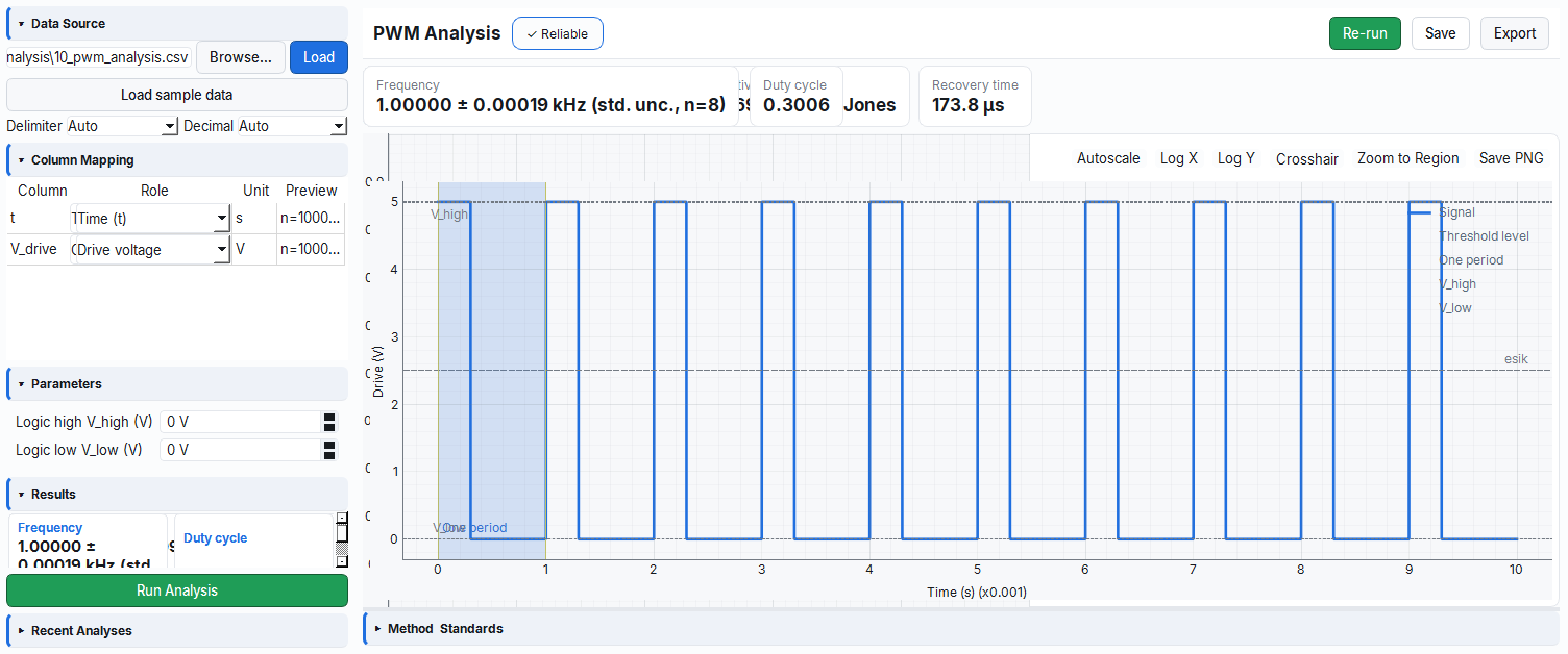
pwm_analysis module — frequency, duty cycle, ripple and THD; phase/delay if a response is present.3. Photovoltaic (PV) Analysis Modules
3.1 MPPT / Fill Factor / PCE — mppt_analysis (Module 11)
It takes how the power produced by a solar cell varies with voltage and quickly answers "at which point does it deliver the most power and what is its efficiency?". Like finding the most efficient gear/pedal speed of a bicycle — a particular point delivers the highest power.
Physical background: A solar cell is a diode in parallel with a light-fed current source; as the voltage rises the diode turns on and swallows part of the current it produces internally. Since power is P = V·I, the power is zero at V=0 (I=I_sc) and again zero at I=0 (V=V_oc); somewhere in between a peak forms — this is the maximum power point (MPP). That is why the P-V curve is a single-peaked hill and you always want to operate the cell at this peak. The fill factor tells you how closely this real peak approaches the ideal "rectangular" power (V_oc·I_sc); the sharper the knee of the J-V curve, the higher the FF.
- Why it is done: to see the cell's maximum power point and overall quality at a quick glance, without going into the detailed engine.
- What it teaches / measures:
p_max_w,v_mpp_v,i_mpp_a= the power at the MPP and the voltage/current that deliver it;v_oc_v/i_sc_a= open-circuit voltage and short-circuit current;fill_factor = P_max/(V_oc·I_sc)= the rectangularity of the curve;pce_pct = P_max/(P_in·A)·100= the power conversion efficiency. - Typical values and interpretation: in a healthy cell FF is 0.7–0.85 (high = low Rs, high Rsh); FF<0.5 indicates high series resistance or low shunt resistance. V_mpp is always below V_oc; FF>1 is physically impossible and indicates that V_oc/I_sc is wrong (the module issues a warning).
- Common mistake / caution: this is the "quick" core — use the detailed
pv_metricsfor Rs/Rsh, the STC badge, and a fine-grid MPP. If the sign convention is wrong, the power peak stays in the negative quadrant and P_max cannot be found; if the incident powerp_in_wand area are not entered, the efficiency for PCE is not computed. - Where it is used: quick solar cell screening, production-line sorting, and educational/lab demonstration.
What it does: Extracts the maximum power point, fill factor and efficiency from a P-V (or I-V) curve (a quick, simple core).
Columns: Required: v, i.
| Parameter | Unit | Description | Default |
|---|---|---|---|
v_oc | V | Open-circuit voltage (from data if 0) | 0.0 |
i_sc | A | Short-circuit current (from data if 0) | 0.0 |
p_in_w | W | Incident power (for PCE) | 0.0 |
cell_area_cm2 | cm² | Cell area | 0.0 |
Applied formula: P = V·I; P_max = max(P) (sign corrected if needed); V_mpp, I_mpp at the MPP; FF = P_max/(V_oc·I_sc); PCE = P_max/(P_in·A)·100.
Outputs: p_max_w, v_mpp_v, i_mpp_a, v_oc_v, i_sc_a, fill_factor, pce_pct. Warning: if FF > 1 check V_oc/I_sc.
Example / expected: 11_mppt_analysis.csv (ideal diode: Isc=30 mA, I0=1 nA, n=1.5). V_oc = V_t·ln(Isc/I0+1) = 0.668 V, FF ≈ 0.80, PCE ≈ 16%.
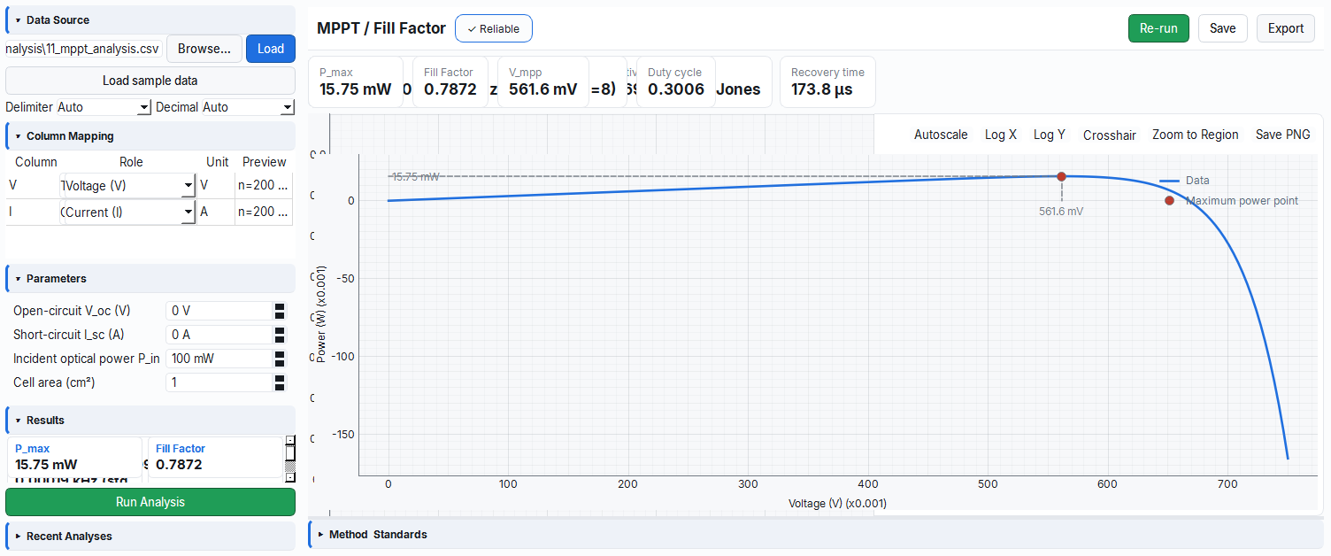
mppt_analysis module — MPP, fill factor and efficiency from the P-V curve.3.2 Solar Cell J-V Metrics — pv_metrics (Module 12)
It computes the entire standard performance report card extracted by applying a voltage to a solar cell and measuring its current (a J-V sweep). Like deriving all of a student's course grades from a single exam — a single sweep gives the cell's full performance table.
Physical background: The illuminated J-V curve is the dark diode curve shifted down by the photocurrent; that is why it takes its characteristic "knee" shape in the fourth quadrant (positive V, negative I — i.e. the power-generating region). The sharpness of the knee depends on two parasitic resistances: the series resistance Rs (contact/grid losses) flattens the slope near V_oc, while the shunt resistance Rsh (leakage/short paths) prevents the slope near V=0 from being steep. The module reads Rs and Rsh from these regional slopes; with the J_sc normalized by area and the PCE computed from the incident power, the result becomes comparable under STC (1000 W/m², 25 °C).
- Why it is done: to document a cell's efficiency and quality in a standards-compliant (IEC), area-normalized and comparable way.
- What it teaches / measures:
v_oc_v= the voltage at which light generation equals the diode loss;j_sc_ma_cm2= the short-circuit current density divided by area;fill_factor= the rectangularity of the knee;pce_pct= efficiency;r_s_ohm= series resistance from the slope above V_oc (low is good);r_sh_ohm= shunt resistance from the slope near V=0 (high is good);metrics_resolved= the reliability flag. - Typical values and interpretation: in a good lab Si cell V_oc ~0.6–0.7 V, J_sc ~30–40 mA/cm², FF 0.75–0.83, PCE ~15%–22%; Rsh should be high (kΩ–MΩ·cm²) and Rs low (<a few Ω·cm²). Low FF + low Rsh = leakage; low FF + high Rs = contact/conduction loss.
- Common mistake / caution: if irradiance/temperature/active_area are not entered, the badge becomes
non_stcand the PCE cannot be compared; if the sign convention is wrong, V_oc/I_sc are found inverted (even though the module auto-detects, do check). Under 1000 W/m², the identityPCE[%] = J_sc·V_oc·FFis a quick way to verify consistency. - Where it is used: solar cell research, pre-certification measurement, and production quality control.
What it does: Computes all performance metrics from a single J-V sweep (parity with the Solarcell 4.8 core).
Columns: Required: v, i.
| Parameter | Unit | Description | Default |
|---|---|---|---|
cell_area_cm2 | cm² | Cell area | 1.0 |
irradiance_w_m2 | W/m² | Irradiance (STC) | 1000.0 |
convention | — | Sign convention (auto/photovoltaic/device) | auto |
v_oc, i_sc | V, A | Manual override | 0.0 |
Applied formula: The sign convention is auto-detected via the power-quadrant integral; V_oc = the persistent first zero crossing of the current; I_sc = the current at V=0; the MPP is the maximum of P=V·I on a fine grid (4000 points).
FF  = P_max / (V_oc · I_sc)
PCE = P_max / P_in · 100,   P_in = E · (A · 1e-4)   [E: W/m², A: cm²]
J_sc = I_sc · 1e3 / A        [mA/cm²]
R_s from a linear fit in the window above Voc [V_oc, V_oc+0.05]; R_sh in the window V=0 ± 0.05 V.
Outputs: v_oc_v, i_sc_a, j_sc_ma_cm2, v_mpp_v, i_mpp_a, p_max_w, fill_factor, pce_pct, r_s_ohm, r_sh_ohm. Flag: metrics_resolved (determines reliability). Provenance conditions: irradiance, temperature, active_area (badge non_stc if missing). Standards: IEC 60904-1, IEC 60904-3, GUM.
Example / expected: 12_pv_metrics.csv (Iph=30 mA/cm², I0=1 nA, n=1.5, Rs=1 Ω, Rsh=10 kΩ, 1 cm² @ 1000 W/m²). J_sc = 30 mA/cm², V_oc ≈ 0.696 V, FF ≈ 0.755, PCE ≈ 15.8%, R_s ≈ 1 Ω, R_sh ≈ 10 kΩ.
PCE[%] = J_sc[mA/cm²]·V_oc[V]·FF holds (the /P_in·100 cancels out); this is a practical way to quickly verify the consistency of FF and PCE.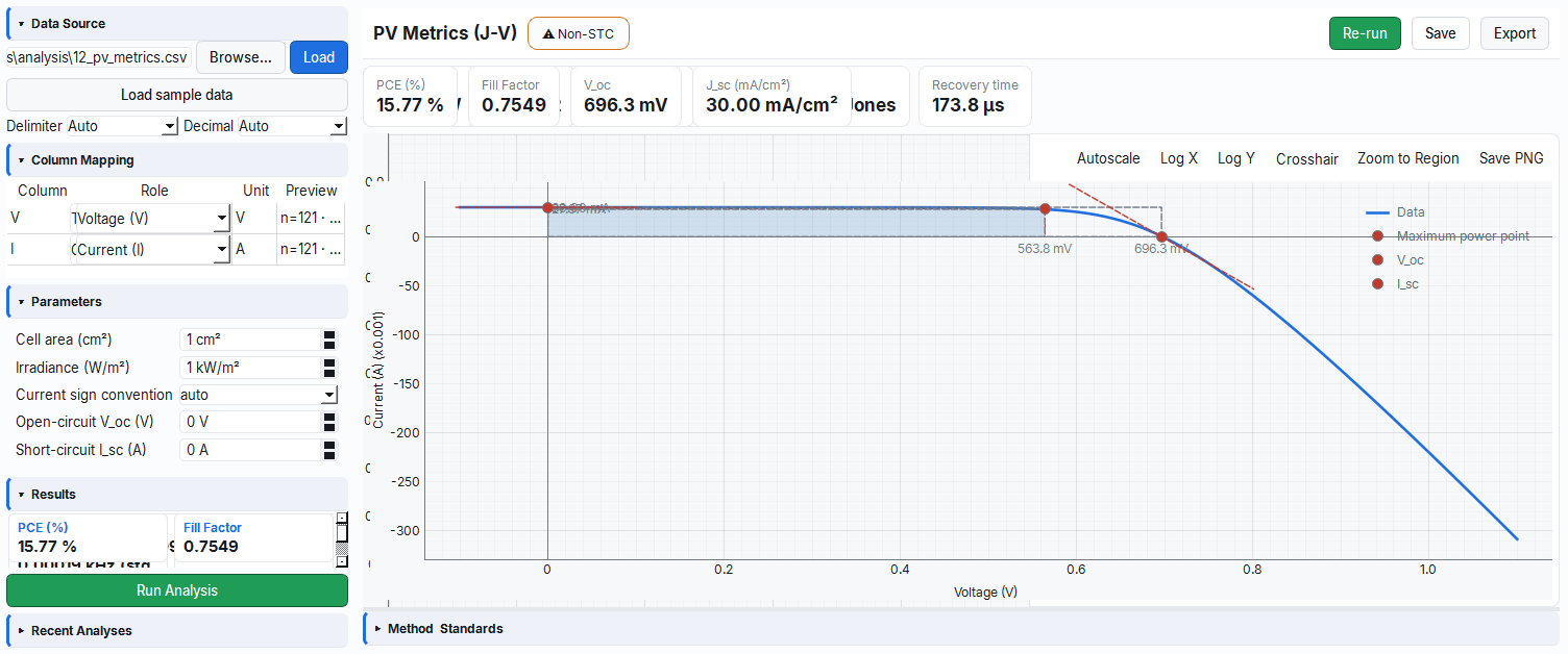
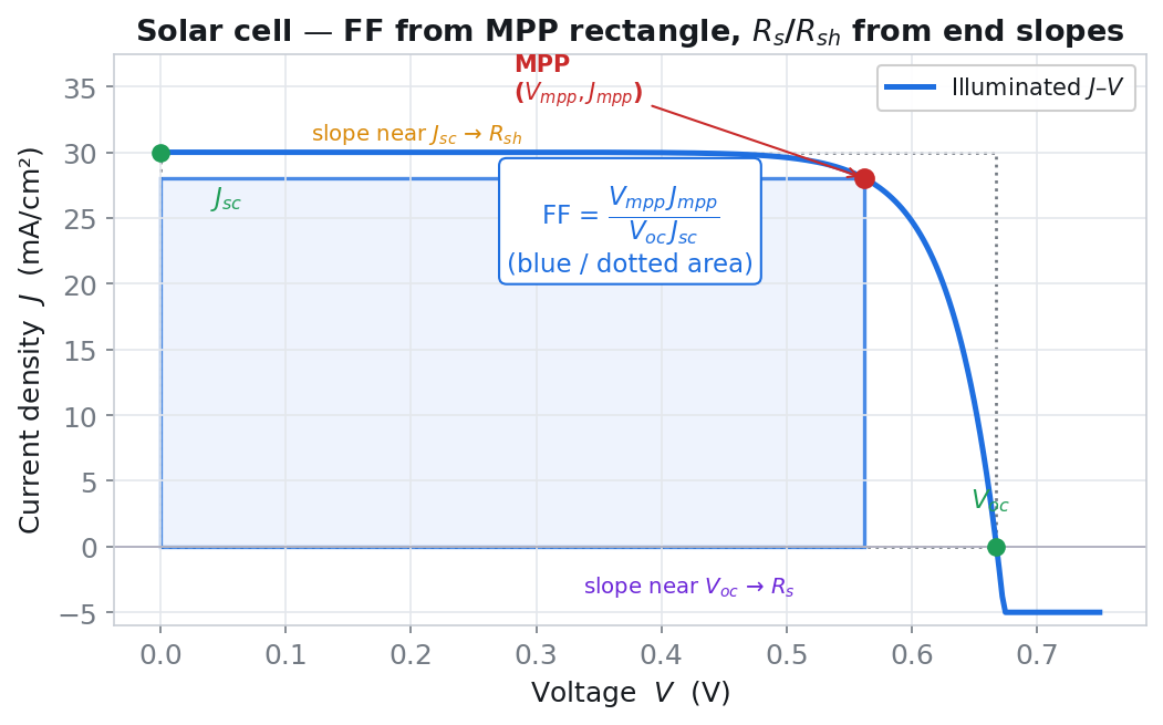
pv_metrics module — V_oc, J_sc, FF, PCE, Rs/Rsh from a single J-V sweep.The illuminated J-V curve is used; the MPP rectangle in the power-generating quadrant and the slopes at the ends are read.
V_oc(the zero crossing of the current) andI_sc(the current at V=0) are marked; the maximum ofP=V·Igives the MPP (V_mpp, I_mpp).- The real MPP rectangle (V_mpp·I_mpp) is ratioed to the ideal
V_oc·I_screctangle. - Result:
FF = P_max/(V_oc·I_sc); the slope nearV_oc→R_s, the slope nearV=0→R_sh.
3.3 J-V Hysteresis — pv_hysteresis (Module 13)
If you sweep the same solar cell in the forward and reverse directions, the two curves usually do not overlap exactly; the difference between them is "hysteresis" and is often a sign of instability. This module converts this difference into a numerical index. Like getting tired differently going up and coming down a hill — if behavior changes with direction, something is shifting.
Physical background: Hysteresis arises from the presence of a slow internal process (especially ion migration in perovskites, plus trap filling/emptying and interface capacitance) that cannot keep up with the sweep. Because these slow charges "catch" the curve at a different place depending on the sweep direction, the forward and reverse J-V curves diverge and an area remains between them; usually the reverse (V_oc→0) sweep gives a better (higher) PCE. The hysteresis index measures this divergence: the PCE-based index quantifies the relative difference between the two efficiencies, while the area-based index quantifies the whole area between the two curves.
- Why it is done: to understand whether the measured efficiency is "real/stable" or misleadingly dependent on the sweep direction and speed, and to assess the device's stability.
- What it teaches / measures:
pce_fwd_pct/pce_rev_pct= the forward and reverse sweep efficiencies;hysteresis_index= the PCE-based index(PCE_rev−PCE_fwd)/PCE_rev;hysteresis_index_area= the normalized area between the two curves. - Typical values and interpretation: in stable Si/inorganic cells HI ≈ 0%–a few %; in perovskites it can be tens of %. A positive and small HI is tolerable; a large HI is a warning that the reported efficiency may be inflated by a single-direction sweep. Ideally, cross-validate with stabilized power output (MPP tracking).
- Common mistake / caution: loading a single-direction sweep and thinking there is "no" hysteresis (the module expects a single bidirectional file); a wrong detection of the turning point distorts the segment split; treating HI as absolute truth without reporting the sweep rate — hysteresis depends on the rate, so devices should not be compared without fixing the rate.
- Where it is used: perovskite/next-generation cell research, stability assessment, and measurement-protocol validation.
What it does: Extracts the mismatch between the forward and reverse sweeps (the hysteresis index).
Columns: Required: v, i (a single bidirectional file). Parameters: cell_area_cm2, irradiance_w_m2, convention.
Applied formula: The voltage turning point splits the data into forward/reverse segments; the PCE is computed for each segment.
HI_PCE  = (PCE_rev − PCE_fwd) / PCE_rev
HI_area = ∫|I_rev − I_fwd| dV / ∫|I_rev| dV      (0..V_oc grid)
Outputs: pce_fwd_pct, pce_rev_pct, hysteresis_index, hysteresis_index_area.
Example / expected: 13_pv_hysteresis.csv (forward I0=2 nA degraded, reverse I0=1 nA). PCE_fwd < PCE_rev, HI ≈ 5% (positive, small).
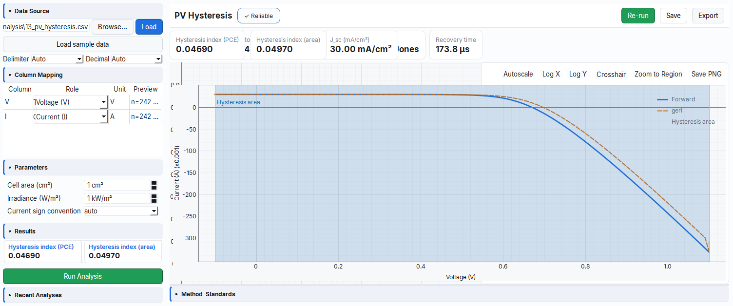
pv_hysteresis module — hysteresis index from the forward/reverse sweep mismatch.3.4 Dark J-V Ideality — pv_diode (Module 14)
By measuring the cell in the dark (no light) and examining its diode-like behavior, it answers "what kinds of losses are inside it?". The ideality factor n is a fingerprint of the recombination mechanism in the cell. Like diagnosing a fault by listening to the engine idle without driving.
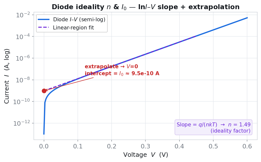
Physical background: In the dark the cell is a pure diode and its forward current rises exponentially with voltage: I = I0·[exp(qV/nkT)−1]. When you plot ln(I) against V, this exponential region turns into a straight line; the slope of the line gives the ideality factor q/(nkT) and the intercept gives the saturation current I0. That is why the mid-voltage region of a semilog J-V should be straight; at very low voltage shunt leakage (Rsh) bends this line from below, and at very high voltage series resistance (Rs) flattens the curve. The module performs the fit exactly in this clean middle window.
- Why it is done: to see the cell's fundamental diode quality and the dominant recombination/loss mechanism independently of light effects.
- What it teaches / measures:
ideality_factor= n, the conduction/recombination fingerprint;saturation_current_a= I0, how much the diode "leaks";r_s_ohm= series resistance at high V;r_sh_ohm= shunt resistance at low V;fit_r2= the quality of the semilog line fit. - Typical values and interpretation: n≈1 diffusion (band-band) dominated, ideal; n≈2 depletion-region (SRH/trap) recombination dominated; 1<n<2 mixed. n>2 indicates a serious defect/interface problem or a poor fit. Low I0 = good diode. The module warns when n∉[0.8,10] or R²<0.98.
- Common mistake / caution: if we move the fit window (
v_fit_min/v_fit_max) into the Rsh-bent or Rs-flattened region, n grows artificially; entering the wrong temperature corrupts the slope→n conversion (thekT/qscale). Read n not on its own but together with R². For physical consistency this module uses theDiodeAnalysisEngine, so there is no metric drift relative to the Diode/Schottky modules. - Where it is used: cell quality diagnosis, identifying loss sources in the production process, and material comparison.
What it does: Extracts the diode ideality factor n, saturation current I0 and Rs/Rsh from the dark J-V. Single physics source: DiodeAnalysisEngine (no metric drift relative to the Diode/Schottky modules).
Columns: Required: v, i.
| Parameter | Unit | Description | Default |
|---|---|---|---|
temperature_k | K | Temperature | 300.0 |
v_fit_min | V | Lower fit bound | 0.05 |
v_fit_max | V | Upper fit bound | 0.5 |
cell_area_cm2 | cm² | Cell area | 1.0 |
Applied formula: Linear fit of ln(I) = ln(I0) + qV/(nkT); slope = q/(nkT) → n; intercept → I0. Rs by the Cheung method, Rsh from the low-V shunt.
Outputs: ideality_factor, saturation_current_a [A], r_s_ohm, r_sh_ohm [Ω], fit_r2. Flag: ideality_resolved. Warning: n ∉ [0.8, 10] or R² < 0.98.
Example / expected: 14_pv_diode_dark.csv (I0=1 nA, n=1.5, Rs=1 Ω, Rsh=1 GΩ; fit 0.05–0.5 V). n = 1.5, I0 = 1 nA, R² ≈ 1.
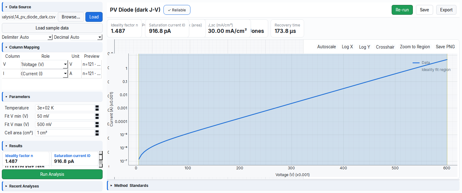
pv_diode module — ideality factor n, I0 and Rs/Rsh from the dark J-V.The dark curve is plotted semi-logarithmically (ln I–V); the exponential region at mid-voltage turns into a straight line.
- An
ln I–Vline is fitted to the clean middle window (v_fit_min..v_fit_max) (the Rsh bend at low V and the Rs flattening at high V are excluded). - The line is extrapolated to
V=0and the saturation current is read from the y-intercept. - Result:
slope = q/(nkT)→n = q/(kT·slope); the intercept →I_0.
3.5 Equivalent Circuit Extraction — pv_equivalent_circuit (Module 14b)
It represents a solar cell with a simple circuit of five fundamental electrical components (a current source, a diode, two resistors) and fits the whole I-V curve to this model simultaneously to find the values of the components in one go. Like redrawing the internal schematic of a complex device from external measurements.
Physical background: The single-diode model describes the cell as follows: light produces a current source Iph, a parallel diode (I0, n) swallows part of it, a shunt resistance Rsh leaks, and a series resistance Rs lowers the output. These five components shape different regions of the same J-V curve (the height of Iph, the diode knee, the Rsh low-V slope, the Rs V_oc slope). Instead of taking regional slopes one by one, the module nonlinearly fits the whole curve to a single equation with the Lambert-W closed-form solution; this way the parameters correctly account for each other's effects and the 1σ uncertainty of each comes out from the fit covariance.
- Why it is done: to explain the cell's behavior not piece by piece (regional slope) but with a holistic and more accurate model, and to know the uncertainty of each parameter.
- What it teaches / measures:
iph_a= the photocurrent source;saturation_current_a(j0_a_cm2) andideality_factor= diode quality;r_s_ohm/r_sh_ohm(area-normalized*_cm2) = the parasitic resistances; in two-diode modei02_a/n2= the second recombination path; for each parameter*_sigma_*= the 1σ uncertainty;fit_r2/rmse_a/nrmse_pct/reduced_chi2= fit quality. - Typical values and interpretation: in a successful fit R²≈1 and the nRMSE is small; if the uncertainties (σ) are small next to the value the parameter is reliable, if large that parameter is not well-constrained by the curve (e.g. at very high Rsh the Rsh σ comes out large — this is normal). It is far more accurate than the slope/ln(I) methods.
- Common mistake / caution: if the initial guess is poor or the data is noisy the fit may get stuck in a local minimum; in that case enable the
robust(global search) option. Forcing a two-diode model on a single curve makes the parameters over-uncertain; read thecircuit_resolvedflag and the σ values together. If the sign convention is wrong the sign of Iph comes out inverted. - Where it is used: advanced cell modeling, simulation (SPICE) parameter extraction, and loss analysis.
What it does: Extracts the Iph, I0, n, Rs, Rsh values SIMULTANEOUSLY by nonlinearly fitting the entire I-V curve to the single-diode (Lambert-W) or two-diode (implicit Newton) model; reports the 1σ uncertainty from the covariance. Far more accurate than the slope/ln(I) methods.
Columns: Required: v, i. Optional: i_dark, t.
| Parameter | Unit | Description | Default |
|---|---|---|---|
model | — | single / two (single/two diode) | single |
fit_mode | — | single_curve / light_dark | single_curve |
cell_area_cm2 | cm² | Cell area | 1.0 |
temperature_c | °C | Temperature | 25.0 |
irradiance_w_m2 | W/m² | Irradiance | 1000.0 |
convention | — | Sign convention | auto |
weighting | — | relative / equal / noise | relative |
robust | bool | Global search + robust fit | False |
Applied formula: The single-diode Lambert-W closed-form solution I(V; Iph, I0, n, Rs, Rsh); five parameters via TRF (trust-region) least-squares. The uncertainties come from the diagonal of the covariance matrix (σ = sqrt(diag)).
Outputs: iph_a, saturation_current_a, ideality_factor, i02_a, n2, r_s_ohm, r_sh_ohm, r_s_ohm_cm2, r_sh_ohm_cm2, fit_r2, rmse_a, nrmse_pct, *_sigma_* for each parameter, j0_a_cm2, reduced_chi2, mae_a, n_points. Flag: circuit_resolved. The result is shown as a drawn equivalent circuit diagram (descriptor circuit_result plot type).
Example / expected: 14b_pv_equivalent_circuit.csv (Iph=30 mA, I0=1 nA, n=1.5, Rs=1 Ω, Rsh=2 kΩ; 298.15 K). All five parameters are fully recovered, R² = 1.
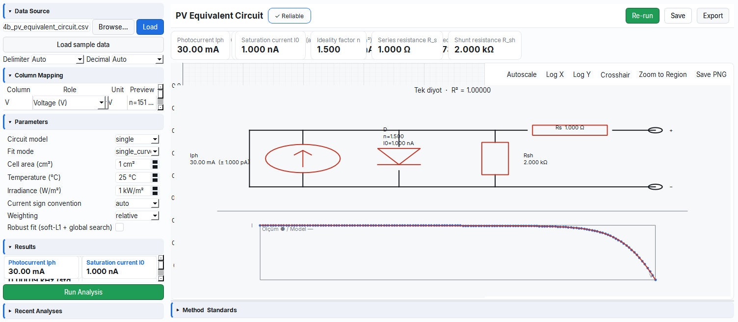
pv_equivalent_circuit module — a five-parameter equivalent circuit diagram via Lambert-W nonlinear fit.Instead of taking a slope/extrapolation from a single region, the entire I-V curve is nonlinearly (least-squares) fitted to the Lambert-W closed-form solution; all five parameters come out at once (more accurate than the ln I–V slope method in 3.4).
- Starting from an initial guess, the
I(V; Iph, I0, n, Rs, Rsh)curve is fitted to all points with TRF. - Result: five parameters +
σ = √diagfrom the covariance (1σ uncertainty); far more accurate than the slope/ln(I) methods.
3.6 Advanced J-V Report (Spec v2.0) — pv_jv_full (Module 15)
It collects in a single package nearly every analysis that can be done from a single J-V file: basic performance, hysteresis, sweep-rate-dependent dynamic effects, diode parameters and shape-distortion (kink/S-curve) diagnostics. Like a vehicle's full inspection report — a check from every angle in one pass.
Physical background: A J-V curve carries not only efficiency but also the charge accumulated during the sweep and the device's internal dynamics. If a time axis is present, the sweep rate comes from the voltage-time slope, and the swept charge and apparent capacitance come from the current-time integral; these dynamic metrics reveal the source of the hysteresis (capacitive/ionic). Furthermore, if there is a step (kink) below the "knee" of the curve or a reverse bend before the MPP (S-shape), this usually indicates that charge extraction is being impeded at an interface (energy barrier, unbalanced transport). Because the module calls the same jv_engine core as the live PV measurement, the report is one-to-one consistent with the real-time measurement.
- Why it is done: to comprehensively document a cell in a single pass and to ensure consistency by using exactly the same engine as the live measurement.
- What it teaches / measures: basic:
v_oc_v,j_sc_ma_cm2,p_max_mw_cm2,fill_factor,pce_pct, window-fittedr_s_a_ohm_cm2/r_sh_a_ohm_cm2; hysteresis packagehi_pce/hi_area_jscvoc/delta_voc_v; dynamicsweep_rate_v_s/charge_density_c_cm2/apparent_cap_mean_f_cm2; diodeideality_factor/j0_a_cm2; diagnosticsrr_at_1v(rectification ratio),j_leak_1v_ma_cm2(leakage),kink_score,s_shape_index. - Typical values and interpretation: in a healthy cell kink_score and s_shape_index ≈0, a high rectification ratio and low leakage are expected; a large s_shape_index/kink indicates a charge-extraction barrier (poor contact/transport layer). The dynamic metrics should shrink at low sweep rate; large apparent capacitance + high HI = ionic/capacitive source.
- Common mistake / caution: feeding a dark curve into the light report makes the metrics "Unreliable" — set the
is_darkflag correctly (the example dataset is precisely the corrected version of this mistake). The dynamic metrics require a time axis (t) orsweep_rate_v_s; otherwise charge/energy/capacitance are not computed. - Where it is used: a detailed research report, problem diagnosis (S-shape, kink, leakage), and full characterization.
What it does: By calling the jv_engine core (the same engine as the live PV measurement), it produces a FULL J-V report: sign convention, V_oc, J_sc/MPP/FF/PCE, window-fitted Rs/Rsh (with R² reported), the forward/reverse hysteresis package, dynamic metrics (sweep rate/charge/energy/apparent capacitance), dark-diode n+J0, rectification ratio/leakage, MPP tolerance window/sharpness, and kink/S-shape diagnostics.
Columns: Required: v, i. Optional: t (the time axis for dynamic analysis).
| Parameter | Unit | Description | Default |
|---|---|---|---|
cell_area_cm2 | cm² | Cell area | 1.0 |
irradiance_w_m2 | W/m² | Irradiance | 1000.0 |
convention | — | Sign convention | auto |
is_dark | bool | Whether it is a dark curve | False |
temperature_c | °C | Temperature | 25.0 |
sweep_rate_v_s | V/s | Sweep rate (from t if absent) | 0.0 |
Outputs (selected): sign_convention; for the primary direction v_oc_v, j_sc_ma_cm2, p_max_mw_cm2, fill_factor, pce_pct, r_s_a_ohm_cm2, r_sh_a_ohm_cm2 (also _fwd/_rev); hysteresis hi_pce, hi_pce_sym, hi_area_jscvoc, a_hyst_mw_cm2, delta_j_max_ma_cm2, delta_voc_v; dynamic sweep_rate_v_s, charge_density_c_cm2, scan_energy_net_mj_cm2, apparent_cap_mean_f_cm2; diode ideality_factor, j0_a_cm2, diode_fit_r2; diagnostics rr_at_1v, rr_max, j_leak_1v_ma_cm2, mpp_window_95_v, kink_score, s_shape_index. Flag: report_resolved.
Example / expected: 15_pv_jv_full.csv (illuminated double sweep, with the application's own column names vds_measured, ids). J_sc = 30 mA/cm², V_oc = 0.696 V, FF = 0.755, PCE = 15.77%; all metrics are resolved. (This dataset is the corrected version of the problem where, in the old screenshot, feeding dark data into the light report made the metrics come out "Unreliable".)
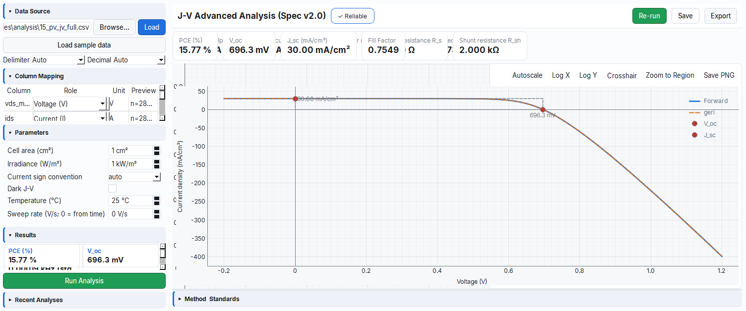
pv_jv_full module — a full J-V report with jv_engine: hysteresis, dynamic metrics, diode and kink/S-shape diagnostics.The FF/Rs/Rsh extraction is exactly the same as in pv_metrics (see 3.2: MPP rectangle + end slopes); this module additionally covers the dark diode and dynamic metrics.
- From the illuminated J-V,
V_oc,J_sc, MPP and Rs/Rsh are read from the slopes at the ends (the same as 3.2). - Result: basic performance (FF, PCE) + hysteresis + dynamic (sweep rate/charge) + dark diode (n, J0) are collected in a single report.
3.7 Stability / Degradation — pv_degradation (Module 16)
It tracks a cell's performance over time and answers "how long does it last?"; it finds the time it takes to drop to a certain percentage of the initial value (T80/T90). Like a phone battery losing capacity over time — the answer to "when does it drop to 80%?".
Physical background: Solar cells degrade over time: moisture/oxygen ingress, light-induced defect formation, ion migration or contact corrosion slowly lower the performance. This decline is often close to an exponential decay; the times to drop to 80% (T80) and 90% (T90) of the initial value are standard lifetime metrics. If the measurement window ends before the device drops to these thresholds, the module uses the slope of the last 30% (if negative) to estimate the threshold by extrapolation — this is why the slope of the observed tail in the plot determines the predicted lifetime.
- Why it is done: to estimate the device's real operating lifetime and to fairly compare the durability of different materials/encapsulations/coatings.
- What it teaches / measures:
initial_value= the mean of the firstn_initialpoints (the reference y0);t80/t90= the times to drop to 80%/90% of y0;retention_pct= the ratio of the last value to y0 (remaining performance);final_value= the last measured value; thet80_extrapolatedflag indicates that the threshold was not measured but estimated. - Typical values and interpretation: in commercial Si modules T80 is decades (~0.5%–1% loss per year); in immature perovskite/organic devices it can be hours–hundreds of hours. High retention = stable device; if
t80_extrapolated=Truethe number was not measured but estimated — be cautious about inferring a long lifetime from a short test. - Common mistake / caution: presenting an extrapolated T80 as precisely as if it were measured; if
n_initialfalls on noisy first points, y0 and therefore all thresholds shift; in non-exponential (stepwise/abrupt) degradation the closed-form τ assumption is misleading. Mind the time unit (s/h). - Where it is used: stability tests (ISOS protocols), product lifetime/warranty estimation, and accelerated aging studies.
What it does: Extracts the T80/T90 lifetime thresholds and the retention percentage from a stability time series (e.g. I_sc(t)).
Columns: Required: t, i. Parameters: n_initial=3 (the number of initial averaging points), extrapolate=True.
Applied formula: y0 = the mean of the first n_initial points; T80 = the first time y drops to 0.80·y0 (linear interpolation; extrapolation if not reached in the data and the last-30% slope is negative); retention = y[-1]/y0·100. Closed form for exponential decay: T80 = −τ·ln(0.80), T90 = −τ·ln(0.90).
Outputs: initial_value, final_value, retention_pct [%], t80, t90 (time unit). Flag: t80_extrapolated. Standard: ISOS 2020.
Example / expected: 16_pv_degradation.csv (I_sc(t)=30 mA·exp(−t/τ), τ=1000 h, 0–500 h). T80 = −τ·ln(0.80) = 223.1 h, T90 = 105.4 h, retention(500 h) = exp(−0.5) = 60.65%.
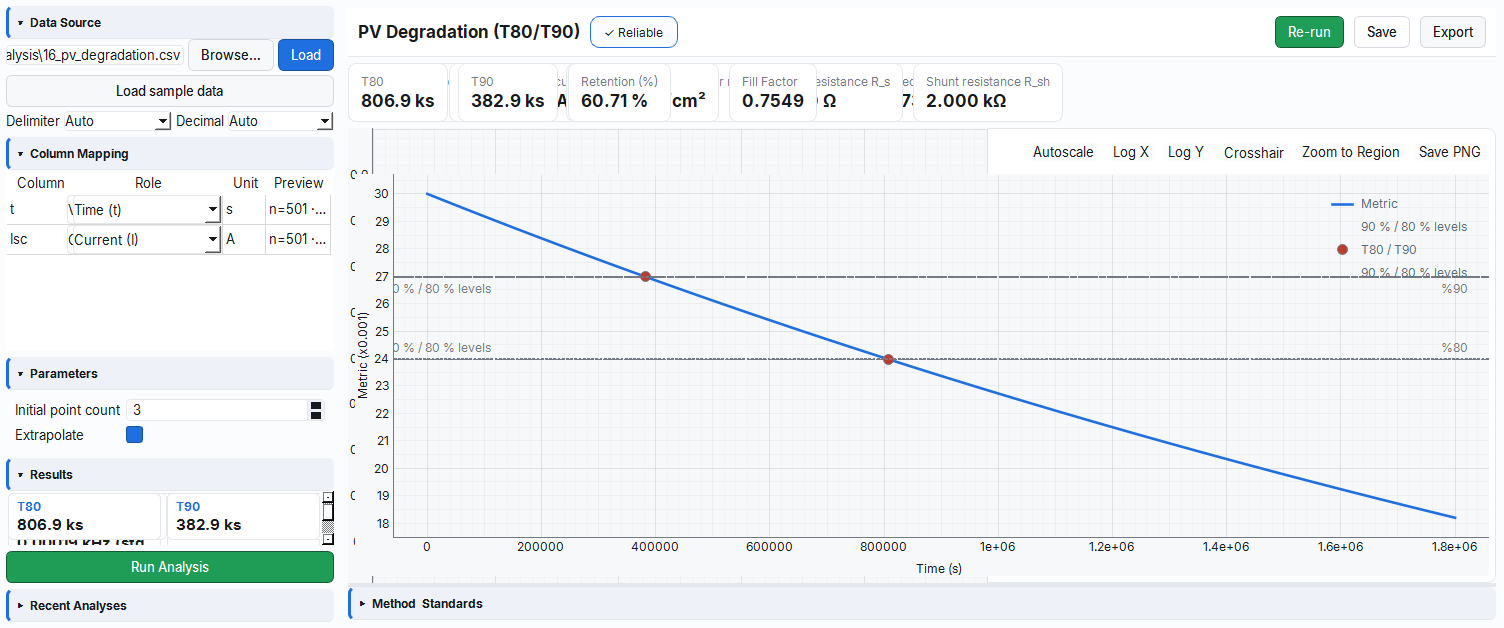
pv_degradation module — T80/T90 lifetime thresholds and retention percentage (ISOS 2020).4. TFT / FET Analysis Modules
4.1 Transfer (On-Off) Curve — tft_on_off (Module 17)
By varying the gate voltage of a thin-film transistor it answers "how good a switch is it?": when does it turn on, how large is the difference between on/off current, how sharply does it switch on. Like measuring at what point a tap starts to flow when you open it, and the difference between fully open and fully closed.
Physical background: The gate voltage Vgs controls the charge density in the channel through the insulating oxide. Below the threshold voltage Vth the channel has not yet formed, so the current flows only by thermal emission and increases exponentially with Vgs — that is why the sub-threshold region of the semilog transfer curve is a straight line and its slope (SS) gives the sharpness of the switching. Above Vth the channel fills and the current now grows linearly/quadratically; this is why the curve settles onto the "on" plateau. The steeper the sub-threshold slope (smaller SS), the fewer the traps; when swept bidirectionally, the shift of the curve (ΔVth) indicates trap filling/emptying hysteresis.
- Why it is done: to quantify the switching quality of the transistor and the electronic properties of the channel/interface material.
- What it teaches / measures:
on_off_ratio= the on/off current ratio (contrast);vth_v= the threshold at which the channel turns on (max-gm tangent extrapolation);ss_mv_dec= the Vgs required to change the current by 10× (switching sharpness/trap indicator);mu_fe_cm2_vs= the field-effect mobility (how easily the carriers flow);dit_cm2_ev= the interface trap density (from SS);vth_y_v/mu0_y_cm2_vs= the Rs-free Y-function extraction;delta_vth_v/hysteresis_window_v= the bidirectional hysteresis. - Typical values and interpretation: for a good TFT on/off ≳10⁶–10⁸; SS ~60–100 mV/dec is near-perfect (60 mV/dec is the room-temperature theoretical limit), >300 mV/dec dense interface traps; mobility varies by technology (a-Si ~1, metal-oxide/IGZO ~10, poly-Si tens of cm²/V·s). A small ΔVth = a stable interface.
- Common mistake / caution: trying to read on/off and SS on a linear axis (it must be semilog); if W/L/C_ox are not entered, mobility and Dit are not computed (but Vth/SS/on-off still come out); reading Ioff from the noise/leakage floor and overstating the on/off (use
ioff_robust_a); missing hysteresis by sweeping a single direction. - Where it is used: display/sensor transistor characterization, evaluation of new semiconductor/dielectric materials, and process quality control.
What it does: Extracts a full parameter report from a transfer curve (Id-Vgs, fixed Vds): on/off ratio, threshold voltage Vth, sub-threshold slope SS, field-effect mobility µFE, Y-function Vth/µ0, interface trap density Dit and (if bidirectional) hysteresis ΔVth. It read-only wraps the SAME engine (calculate_transfer_summary) as the measurement side.
Columns: Required: v (Vgs), i (Id).
| Parameter | Unit | Description | Default |
|---|---|---|---|
w_um | µm | Channel width W | 100.0 |
l_um | µm | Channel length L | 10.0 |
cox_nf_cm2 | nF/cm² | Gate oxide capacitance C_ox | 34.5 |
fixed_vds | V | Fixed Vds | 1.0 |
method | — | Linear / Saturation | Linear |
Applied formula:
I_on/I_off = max|I_d| / min|I_d|
SS         = dV_gs / d(log10 I_d)              (steepest sub-threshold window)
µ_FE       = g_m · L / (W · C_ox · V_ds)       (linear region, max-gm)
V_th       = V_gs* − I_d* / g_m,max            (max-gm tangent extrapolation)
Outputs: on_off_ratio, vth_v, ss_mv_dec, mu_fe_cm2_vs, ion_a, ioff_a, ioff_robust_a, on_off_ratio_robust, gm_max_s, gm_max_vgs_v, ss_r2, vth_y_v, mu0_y_cm2_vs, y_r2, dit_cm2_ev, vth_fwd_v, vth_bwd_v, delta_vth_v, hysteresis_window_v, extraction_method. Flag: analysis_resolved. Standards: IEEE 1620-2008, GUM.
Example / expected: 17_tft_on_off.csv (n-type sigmoid, Vds=1 V). I_on/I_off ≈ 1e8, V_th ≈ 0.75 V, SS ≈ 0.15·ln10·1000 = 345 mV/dec.
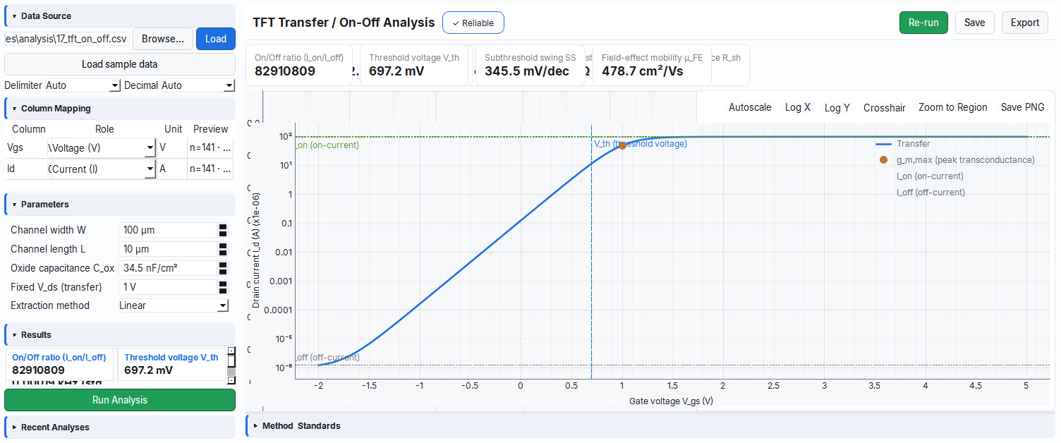
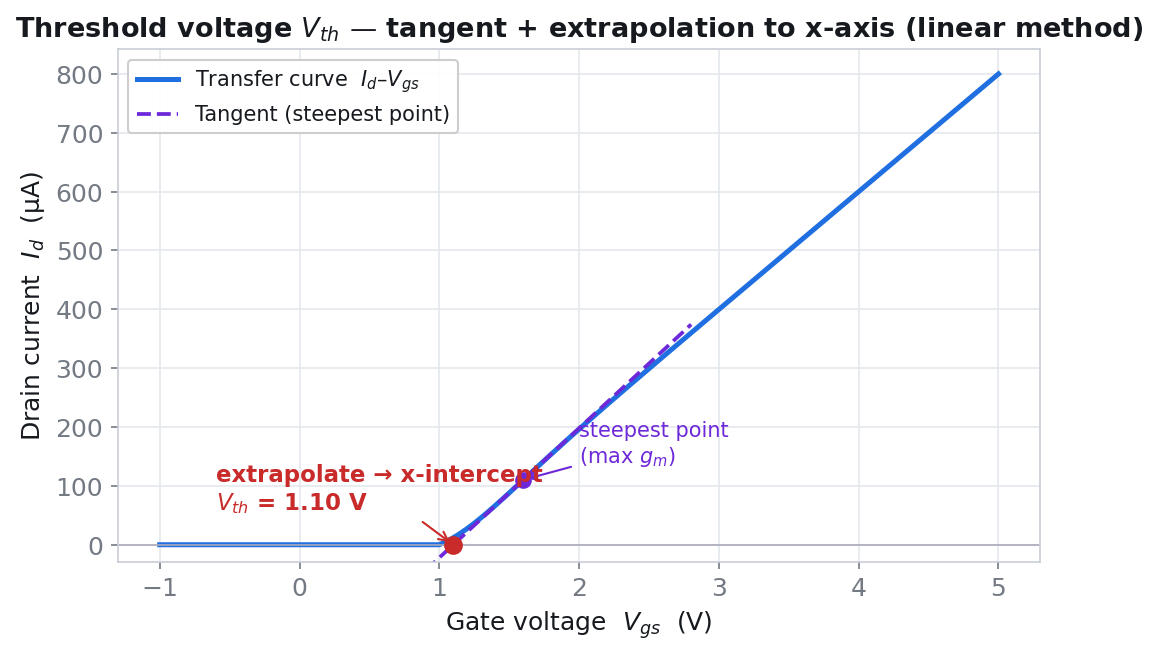
tft_on_off module — on/off ratio, Vth, SS, µFE, Y-function, Dit and hysteresis.The linear transfer curve (I_d–V_gs) is used; a tangent is drawn at the steepest-slope (max-gm) point.
- The point where
g_m = dI_d/dV_gsis maximum is found and a tangent line is drawn there. - The tangent is extended to the x-axis (I_d=0); the intercept gives the threshold voltage.
- Result:
V_th = V_gs* − I_d*/g_m,max(the x-intercept). Mobility from the same slope:µ_FE = g_m·L/(W·C_ox·V_ds).
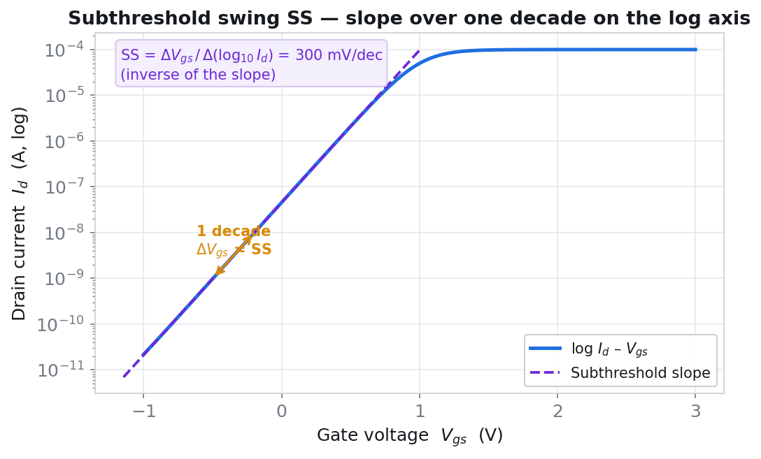
The transfer curve is plotted semi-logarithmically (log I_d–V_gs); the steepest linear portion in the sub-threshold region is selected.
- A slope is fitted to the steepest line segment of one decade (where the current changes by ×10) in the sub-threshold region.
- The ΔV_gs required for that one decade is read.
- Result:
SS = ΔV_gs/Δ(log10 I_d)[mV/dec] (the inverse of the slope); small SS = sharp switching.
4.2 Output Curve — tft_output (Module 18)
With the transistor on, it examines how much current it can drive as the drain voltage is increased and where the current "saturates" and stabilizes. Like measuring how much flow a water pump can deliver as the pressure increases and where it hits the ceiling.
Physical background: At low Vds the channel is conductive everywhere and the current increases linearly with Vds (linear/triode region, slope ≈ 1/Ron). As Vds grows the channel is "pinched off" at the drain end (pinch-off); beyond this point the extra Vds mainly drops across the pinched region and the current is nearly constant — the saturation region. This is the reason for the gentle plateau of the curve. The plateau is not perfectly flat: due to channel-length modulation (λ) it rises slightly; this slope is read as the output resistance r_o = 1/(I_dsat·λ) and the Early voltage V_A = 1/λ. For multiple Vgs, this family of curves also gives the saturation mobility.
- Why it is done: to understand the current the transistor can drive, the output resistance and the gain potential as an amplifier (intrinsic gain).
- What it teaches / measures:
ron_ohm= the linear-region on-resistance (low-Vds slope);idsat_a= the saturation current;lambda_per_v= channel-length modulation;output_resistance_ohm= the output resistance r_o in saturation;va_v= the Early voltage (1/λ);av= the intrinsic gain g_m·r_o;knee_v= the linear→saturation knee voltage; if multiple Vgs are presentmu_sat_cm2_vs= the saturation mobility;n_curves/vgs_used_v= the number of curves in the family. - Typical values and interpretation: low Ron = good drive capability; high r_o / high V_A (large 1/λ) = a flat plateau, a good current source and high gain; low V_A (steep plateau) = a short-channel effect. The knee voltage is roughly around Vgs−Vth.
- Common mistake / caution: the saturation mobility cannot be extracted from a single curve (single Vgs) (
µ_sat = N/A); fitting λ from the linear region instead of the plateau ruins r_o; reading Ron from the saturation region. r_o, λ and V_A are different expressions of the same physics and must be consistent. - Where it is used: transistor modeling for circuit design, sizing the driver/amplifier stage, and performance validation.
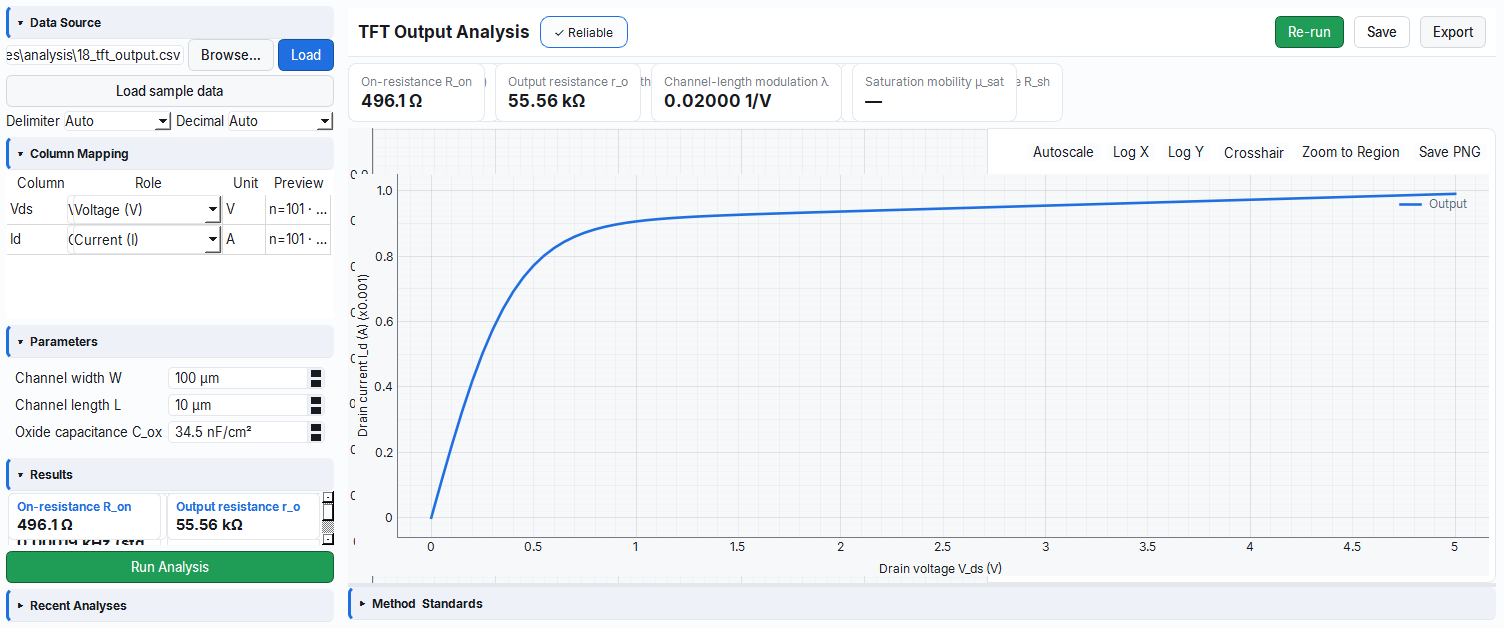
What it does: Extracts Ron, output resistance r_o, channel-length modulation λ, Early voltage VA, Idsat, knee and (if multiple Vgs are present) saturation mobility µ_sat from an output curve/family (Id-Vds, stepped Vgs). It read-only wraps the measurement engine analyze_iv.
Columns: Required: v (Vds), i (Id). Optional: v_bias (stepped Vgs step axis). Parameters: w_um=100, l_um=10, cox_nf_cm2=34.5.
Applied formula: Saturation region I_d = I_dsat·(1 + λ·V_ds); output resistance r_o = 1/(I_dsat·λ); Ron from the low-Vds slope; Early voltage V_A = 1/λ.
Outputs: ron_ohm, output_resistance_ohm, lambda_per_v [1/V], mu_sat_cm2_vs, va_v, idsat_a, gm_s, av, knee_v, vth_sat_v, mu_sat_r2, vgs_used_v, n_curves. Flag: analysis_resolved.
Example / expected: 18_tft_output.csv (single curve Vgs=4 V, λ=0.02/V). I_dsat = 1e-4·(4−1)² = 9e-4 A, λ = 0.02/V, r_o = 1/(I_dsat·0.02) ≈ 5.6e4 Ω, R_on ≈ 4.4e2 Ω. Since it is a single curve, µ_sat = N/A.
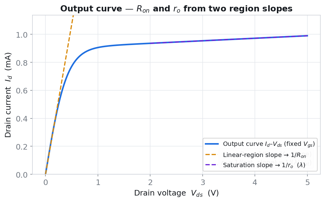
tft_output module — Ron, r_o, λ, Early voltage VA, Idsat and saturation mobility.The output curve (I_d–V_ds) is used; the slope of two different regions is taken.
- A line is fitted to the low-V_ds (linear/triode) region; its slope gives
1/R_on. - The line
I_d = I_dsat·(1 + λ·V_ds)is fitted to the gentle slope of the saturation plateau. - Result:
R_on = 1/slope_linear; from the saturation sloper_o = 1/(I_dsat·λ)andV_A = 1/λ.
5. Statistics and Endurance Modules
5.1 Descriptive Statistics — descriptive_stats (STAT-01)
When you measure the same thing repeatedly the results do not come out exactly identical; this module computes from those repetitions the mean, the spread and the scientific answer to "how much can I trust the mean?" (the uncertainty). Like shooting the same arrow at a target many times and looking at how scattered the shots are — if the spread is narrow your confidence is high. This is a pure statistics module; it has no device-specific physics.
- Why it is done: to quantify the repeatability of a measurement and to report the result with a standard uncertainty (GUM).
- What it teaches / measures:
mean/median= central tendency;std_sample= spread;u_mean = s/√N= the standard uncertainty of the mean;expanded_u_mean = k·u= the expanded uncertainty;rel_std_pct= the relative scatter. - Common mistake / caution: with few repetitions (
2 ≤ N < 10) the uncertainty is weak; with a single measurement (N=1) the uncertainty is undefined (the badge is unreliable). Do not confuse the standard deviation (spread) with the uncertainty of the mean (smaller by √N). - Where it is used: measurement uncertainty budget, calibration report, quality-control statistics.
What it does: Extracts descriptive statistics and the Type-A standard uncertainty of the mean from repeated measurements (a single numeric column).
Columns: Required: i (or v if absent). Parameter: coverage_k=2.0 (coverage factor, 1–6).
Applied formula (GUM Type-A):
s              = std(x, ddof=1)         (sample standard deviation, Bessel)
u(x̄)           = s / sqrt(N)            (standard uncertainty of the mean)
U              = k · u(x̄)               (expanded uncertainty)
rel_std_pct    = 100 · s / |x̄|
Outputs: n, mean, median, min, max, range, std_sample, u_mean, coverage_k, expanded_u_mean, rel_std_pct. Flag: enough_points (N ≥ 2, determines reliability). Warning: if 2 ≤ N < 10 the uncertainty rests on few repetitions (weak). Standards: ISO/IEC Guide 98-3 (GUM), NIST/SEMATECH e-Handbook.
Example / expected: 19_descriptive_stats.csv (I = 1..11 A, N=11). mean = median = 6, range = 10, s = sqrt(110/10) = sqrt(11) = 3.31662, u(mean) = sqrt(11)/sqrt(11) = 1.0, U = 2·1.0 = 2.0 (k=2).
u_mean output of this module can be fed as a Type-A input into the GUM uncertainty framework in the Calc workspace; this way a combined uncertainty budget can be built.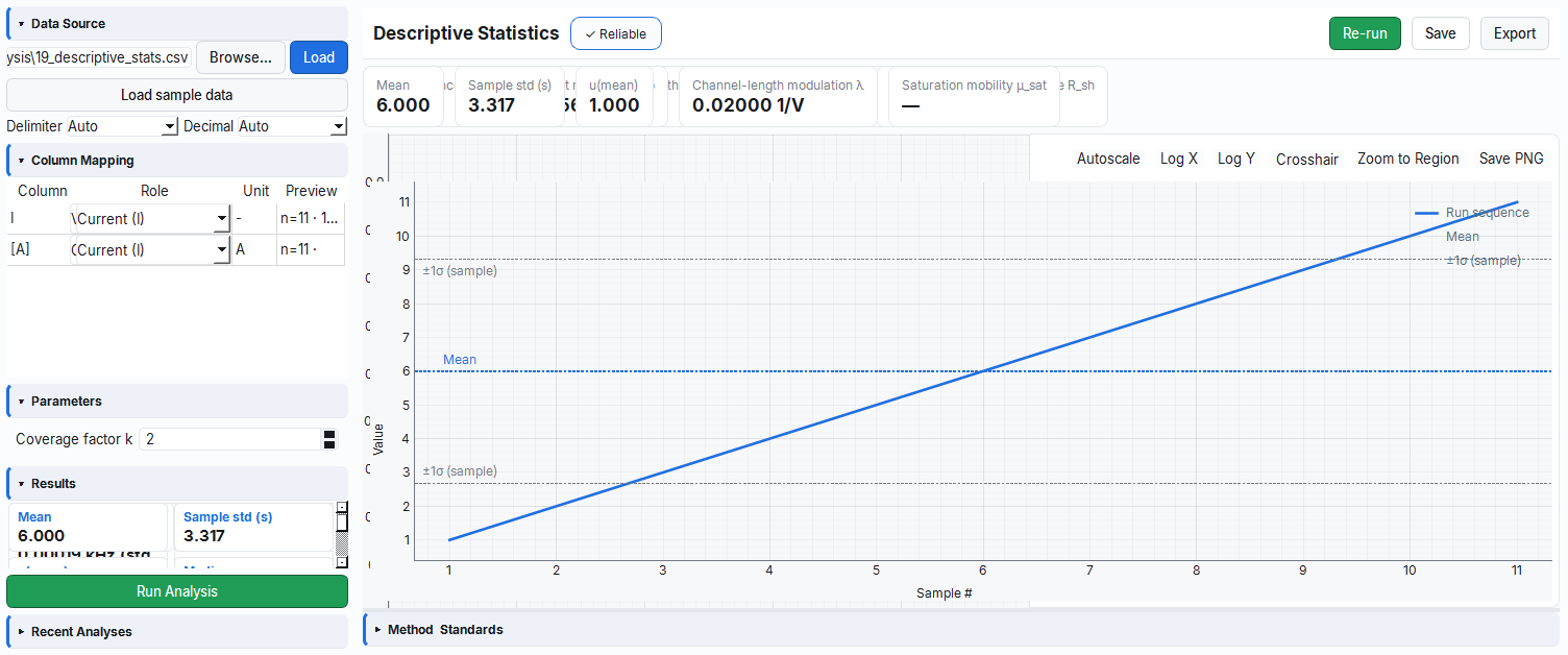
descriptive_stats module — descriptive statistics and GUM Type-A standard uncertainty.No plot is required; it is computed directly by formula from the scatter of the repeated measurements.
- The sample standard deviation
s = std(x, ddof=1)(Bessel correction) is found. - Result: the uncertainty of the mean
u(x̄) = s/√N; expandedU = k·u(x̄).
5.2 Linear Regression — linear_regression (STAT-02)
If there is a straight proportionality between two quantities (e.g. if current increases as light increases), this module draws the "best line" through the points and gives the slope/intercept along with their reliability. Like passing the most suitable line through the middle of scattered points with a ruler — but with mathematics, not by eye. This is a pure statistics (OLS) module; it has no device-specific physics.
- Why it is done: to quantify the relationship between two variables, to extract a calibration line, or to derive a physical quantity from a slope.
- What it teaches / measures:
slope/intercept= the slope and intercept of the line (each with a Type-Au_*and expanded uncertainty);r_squared= the fit quality;residual_std= the scatter of the residuals. - Common mistake / caution: with few points (
N < 8) the uncertainties are wide; mistaking a high R² for "proof of linearity" (a curve can also give a high R² — look at the residuals); in a perfect fit (R²=1) the uncertainty comes out 0, which is a sign of synthetic data. - Where it is used: sensor calibration, trend analysis, experimental-law validation.
What it does: Applies linear least-squares (OLS) to an (x, y) pair; gives the slope/intercept and their Type-A uncertainties.
Columns: Required: v (x), i (y). Parameter: coverage_k=2.0.
Applied formula:
slope m   = Σ(x−x̄)(y−ȳ) / S_xx,    S_xx = Σ(x−x̄)²
intercept b  = ȳ − m·x̄
R²       = 1 − SS_res / SS_tot
s²       = SS_res / (N−2)                  (residual variance, N−2 degrees of freedom)
u(m)     = sqrt( s² / S_xx )
u(b)     = sqrt( s² · (1/N + x̄²/S_xx) )
Outputs: n, slope, u_slope, expanded_u_slope, intercept, u_intercept, expanded_u_intercept, coverage_k, r_squared, residual_std. Flag: good_fit (R² > 0.99). Warning: if N < 8 the uncertainties are weak/wide.
Example / expected: 20_linear_regression.csv (exact line y = 3x + 2, x=0..9). slope = 3, intercept = 2, R² = 1, residual_std = 0 → u(slope) = u(intercept) = 0 (perfect fit).
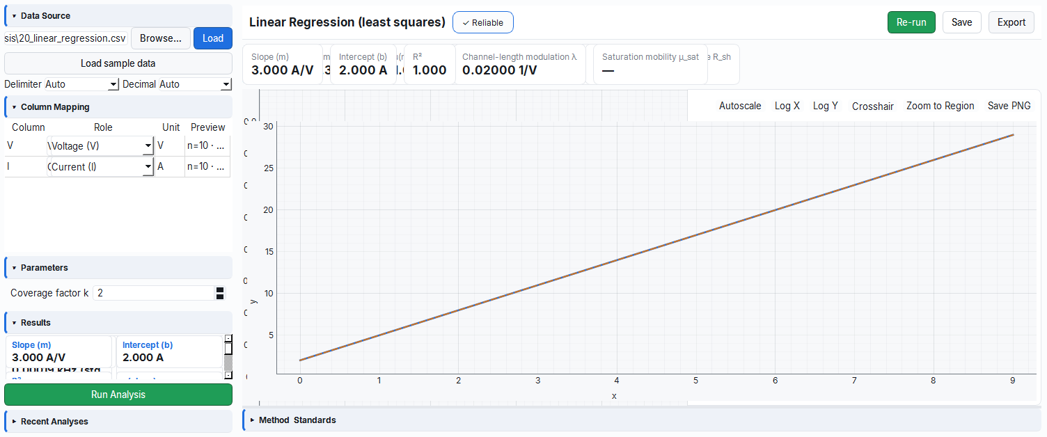
linear_regression module — OLS slope/intercept and their Type-A uncertainties.A least-squares line is fitted to the (x, y) points; the slope, intercept and the uncertainty from the residuals come out.
- The line that minimizes the sum of squared residuals is fitted to the points; slope
m = Σ(x−x̄)(y−ȳ)/S_xx. - The line is extended to the y-axis and the intercept
b = ȳ − m·x̄is read. - Result: from the scatter of the residuals,
u(m) = √(s²/S_xx)andu(b)(Type-A uncertainty).
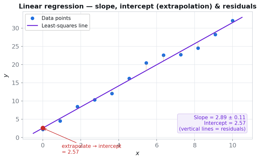
5.3 Endurance (Resistive Switching) — endurance (Module 36)
How many "write-erase" cycles can a resistive-switching memory (memristor) cell withstand? This module tracks the high and low resistance states in each cycle and finds when the "window" between them begins to close (failure). Like switching a light switch on and off thousands of times and counting when it starts to stick.
Physical background: An RRAM cell stores "1" and "0" by forming (SET → low resistance, LRS) or rupturing (RESET → high resistance, HRS) a conductive filament inside it. To read the data the resistances of the two states must be clearly different; this difference is the "memory window" ratio R_HRS/R_LRS. As the cycles repeat, the filament material fatigues (ion depletion, thermal damage): LRS rises or HRS drops and the window narrows. When the window falls below a certain threshold the two states can no longer be safely distinguished — this is the endurance failure. That is why the cycle-resistance plot is drawn semilog and the moment the two series approach each other is sought.
- Why it is done: to assess the lifetime of a memory cell (number of cycles) and its ability to reliably distinguish the states.
- What it teaches / measures:
window_ratio_initial/window_ratio_final/window_ratio_min= the start, end and worst of the window ratio R_HRS/R_LRS;first_failure_cycle= the first cycle where the window drops below the threshold (none if no failure);r_lrs_final_ohm/r_hrs_final_ohm= the final state resistances;n_cycles_analyzed= the number of cycles analyzed;endurance_pass= the decision of no failure AND worst window ≥ threshold. - Typical values and interpretation: in a robust cell the window ratio is ≳10 (usually 10–100+) and stays stable across the cycles; the first cycle that drops below
failure_window_ratio(default 5) is the end of life. A high and narrowly-distributed window is good; a window that drops or scatters heavily with cycling is a sign of fatigue/instability. - Common mistake / caution: mind the role overloading — here
i= R_LRS,v= R_HRS,t= the cycle number (not current/voltage); if R_HRS is not loaded only LRS is computed and a missing-HRS note is left (the window ratio is not produced). Looking linear instead of semilog hides small LRS changes. - Where it is used: next-generation memory (RRAM/memristor) research, reliability/endurance testing, and material/structure comparison.
What it does: Extracts resistive-switching memory metrics from a wide-format endurance dataset (one row per SET/RESET cycle).
Columns (role overloading — Phase 1 contract): Required: t (cycle number), i (R_LRS, the low-resistance state). Optional: v (R_HRS, the high-resistance state). Parameter: failure_window_ratio=5.0 (failure threshold, lower bound 1.0).
Applied formula:
window ratio   W = R_HRS / R_LRS
first failure  = the first cycle number satisfying W < threshold
Outputs: window_ratio_initial, window_ratio_final, window_ratio_min, first_failure_cycle, r_lrs_final_ohm, r_hrs_final_ohm [Ω], n_cycles_analyzed. Flag: endurance_pass (NO failure and worst window ≥ threshold). If R_HRS is not loaded, an LRS-only computation is done and a missing-HRS note is left.
Example / expected: 36_endurance.csv (40 healthy cycles; R_LRS ≈ 1 kΩ ±3%, R_HRS ≈ 100 kΩ ±5%). Window ≈ 100 (min ≈ 93.6) ≫ threshold 5.0 → no first failure, endurance_pass = True. Final R_LRS ≈ 1027 Ω, final R_HRS ≈ 104219 Ω. A semilog R-cycle plot is drawn (LRS primary, HRS secondary series).
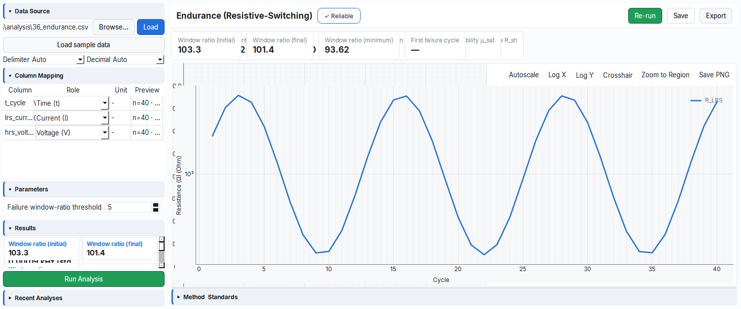
endurance module — per-cycle resistance window and failure-cycle detection.6. Reliability Badge and Quality Flags — Quick Reference
The table below summarizes each module's main reliability-determining flag and its standard references. If the badge comes out unreliable, first check this flag; if it comes out non_stc, enter the relevant condition parameter (irradiance / temperature / active_area).
| Module | Main flag (sets_reliability) | Extra quality/warning | Standard |
|---|---|---|---|
temporal_response | cycles_found, above_floor | nyquist_ok | IEEE 181, IEC 60469, GUM |
photo_dark_ratio | dark_current_resolved | — | — |
persistence | (R²-based) | R² < 0.95 warning | JEDEC BTI (convention) |
bandwidth_3db | rise_time requirement | — | — |
responsivity | i_photo resolution | spot>area warning | IEC 60904-8 |
eqe_iqe | R/λ requirement | EQE/IQE>100% warning | — |
linearity_ldr | powerlaw fit | R² < 0.999 warning | IEC 60904-10 |
nep_detectivity | nep_reliable | D* > 1e14 warning | GUM |
noise_psd | PSD resolution | — | — |
pwm_analysis | period count | — | — |
mppt_analysis | MPP resolution | FF > 1 warning | — |
pv_metrics | metrics_resolved | FF ≤ 1; non_stc conditions | IEC 60904-1/3, GUM |
pv_hysteresis | segment split | — | IEC 60904-1 |
pv_diode | ideality_resolved | n∉[0.8,10], R²<0.98 | — |
pv_equivalent_circuit | circuit_resolved | fit convergence | — |
pv_jv_full | report_resolved | report warnings | IEC 60904-1/3 |
pv_degradation | retention resolution | t80_extrapolated | ISOS 2020 |
tft_on_off | analysis_resolved | SS > 0 | IEEE 1620, GUM |
tft_output | analysis_resolved | — | IEEE 1620 |
descriptive_stats | enough_points (N≥2) | N ≥ 10 | GUM |
linear_regression | good_fit (R²>0.99) | N ≥ 8 | GUM |
endurance | endurance_pass | missing-HRS note | — |
7. Example Datasets and Expected Results — Summary
All example files are under examples/analysis/; each one can be loaded directly in the Analyze workspace (columns are auto-mapped) or regenerated and verified with python -m examples.analysis.generate_and_verify.
| File | Module | Expected main result |
|---|---|---|
01_temporal_response.csv | temporal_response | t_rise=43.944 µs, t_fall=131.833 µs, 3 cycles |
02_photo_dark_ratio.csv | photo_dark_ratio | ratio=99.0, SNR=59.91 dB |
03_persistence_decay.csv | persistence | τ=0.25 s, R²≈1 |
04_bandwidth_3db.csv | bandwidth_3db | BW=7964.9 Hz |
05_responsivity.csv | responsivity | R=0.45 A/W, EQE 65.6% |
06_eqe_iqe.csv | eqe_iqe | EQE=65.64%, IQE=72.94% |
07_linearity_ldr.csv | linearity_ldr | α=1.0, LDR=100 dB, C=0.45 |
08_nep_detectivity.csv | nep_detectivity | D*≈1e12 Jones |
09_noise_psd.csv | noise_psd | γ=1.0, f_c=200 Hz, floor=1e-22 |
10_pwm_analysis.csv | pwm_analysis | f=1000 Hz, duty=30% |
11_mppt_analysis.csv | mppt_analysis | V_oc=0.668 V, FF≈0.80, PCE≈16% |
12_pv_metrics.csv | pv_metrics | J_sc=30, V_oc=0.696, FF=0.755, PCE=15.8% |
13_pv_hysteresis.csv | pv_hysteresis | HI≈5%, forward worse |
14_pv_diode_dark.csv | pv_diode | n=1.5, I0=1 nA |
14b_pv_equivalent_circuit.csv | pv_equivalent_circuit | Iph=30 mA, I0=1 nA, n=1.5, Rs=1, Rsh=2k, R²=1 |
15_pv_jv_full.csv | pv_jv_full | J_sc=30, V_oc=0.696, FF=0.755, PCE=15.77% |
16_pv_degradation.csv | pv_degradation | T80=223.1 h, T90=105.4 h, retention=60.65% |
17_tft_on_off.csv | tft_on_off | on/off≈1e8, V_th≈0.75 V, SS≈345 mV/dec |
18_tft_output.csv | tft_output | I_dsat=9e-4 A, λ=0.02/V, r_o≈5.6e4 Ω |
19_descriptive_stats.csv | descriptive_stats | mean=6, s=3.31662, u=1.0, U=2.0 |
20_linear_regression.csv | linear_regression | slope=3, intercept=2, R²=1 |
36_endurance.csv | endurance | window≈100, no failure, pass=True |
example_specs.py and is verified separately for both the numerical expectations (value + tolerance) and the physical laws (e.g. FF ≤ 1, EQE ≤ 100%, V_mpp < V_oc, t_fall/t_rise = τ_f/τ_r, D* > 0). This way each metric both produced the correct number and did not violate the physics.