LCR/Impedance and RPS/RUS Analyses

This section covers two advanced module families found in the Analysis workspace: the capacitance–voltage and impedance-based LCR/Impedance family, and the resonant piezoelectric/ultrasound-based RPS/RUS family. Both families extract semiconductor, thin-film, photovoltaic and elastic device parameters from the measurement files you upload, completely, with an uncertainty budget and in a reproducible manner.

LCR / Impedance family (A1–A8): Extracts semiconductor/thin-film/photovoltaic device parameters (carrier density, built-in voltage, trap energies, interface trap density, recombination lifetime) from capacitance–voltage (C–V), capacitance–frequency (C–f), impedance spectroscopy (Z–f) and temperature-resolved admittance (TAS) data.
RPS / RUS family (29–35): Extracts resonance frequency, quality factor, acoustic attenuation, relative piezoelectric response, nonlinearity ratio, relative elastic modulus and the full elastic tensor (C_ij) from resonant piezoelectric spectroscopy (RPS) and resonant ultrasound spectroscopy (RUS) data.

Both families are computed in the application's Qt-free core engines (app/analysis_kit/engines/lcr and .../rps); the numbers are produced from a single source and the visual layer never recomputes. Uncertainties are propagated from the fit covariance within the GUM (JCGM 100:2008) framework.

ℹ️

Note In these modules data columns are read by name (no role assignment needed). As long as an LCR/RPS file carries the correct column names (e.g. bias_v, cp_f, freq_hz, z_re_ohm, harmonic, r_v, t_set_k), it is computed directly without manual column mapping.

Analysis workspace main screen, list of LCR and RPS modules — **Figure.** The Analysis workspace; LCR/Impedance and RPS/RUS modules are selected here.

🎓 What is it for? — The Analysis workspace: extracting device parameters from a file

This section describes two analysis families that take the raw measurement files (CSV) you recorded in the lab and extract meaningful numbers about the material and device from them. Just as a doctor looks at an X-ray film and says "the bone is this dense," the software looks at your curves and reads physical quantities such as carrier density, trap energy or elastic modulus.

Why it's done: Raw curves (capacitance, impedance, resonance peaks) cannot be interpreted on their own; analysis converts them into comparable physical parameters.
What it teaches / measures: Each module produces a specific quantity (e.g. carrier density, lifetime, elastic constants) and gives its uncertainty (± error) alongside it.
Where it's used: Semiconductor/solar cell research, thin-film quality control, materials characterization and failure analysis.

Common Concepts

Data columns and unit notation

The LCR/RPS example files carry the unit in square brackets in their CSV headers; the loader strips the trailing [unit] suffix and binds the column by name. Typical headers:

Mode	CSV column header (example)	Description
C–V	`bias_v [V], cp_f [F], rp_ohm [ohm], g_s [S], z_re_ohm [ohm], z_im_ohm [ohm]`	Fixed frequency, swept DC bias
C–f	`freq_hz [Hz], cp_f [F], g_s [S], rp_ohm [ohm], z_re_ohm [ohm], z_im_ohm [ohm]`	Fixed bias, log-swept frequency
Z–f	`freq_hz [Hz], z_re_ohm [ohm], z_im_ohm [ohm], z_mag_ohm [ohm], z_phase_deg [deg], bias_v [V]`	Impedance spectroscopy
TAS	`temperature_k [K], freq_hz [Hz], cp_f [F], g_s [S]`	One C–f sweep stacked at each temperature
RPS	`harmonic, freq_hz [Hz], x_v [V], y_v [V], r_v [V], t_set_k [K]`	Lock-in harmonic/phase output

✅

Tip Metadata (device area, temperature, device type) is not carried via the CSV. Therefore values the engine needs, such as area_cm2, temperature_k, eps_r, must be supplied either from the relevant column in the file or from the module parameter panel. The example files map these values via parameter defaults.

Physical constants (CODATA 2019, SI)

Constant	Symbol	Value
Elementary charge	q	1.602176634 × 10⁻¹⁹ C
Boltzmann constant	k_B	1.380649 × 10⁻²³ J/K
Boltzmann (eV)	k_B	8.617333262 × 10⁻⁵ eV/K
Vacuum permittivity	ε₀	8.8541878128 × 10⁻¹² F/m

Uncertainty and goodness-of-fit metrics

All standard uncertainties are k = 1 (expanded uncertainty is not separately reported; project convention).
For linear fits the uncertainty is computed from the numpy.polyfit covariance matrix; for nonlinear fits (scipy.optimize.least_squares) from the Jacobian with a-posteriori s² scaling.
r2 (coefficient of determination) is reported for every fit; each module also returns an analysis_resolved flag (False when it cannot be resolved).

⚠️

Warning The impedance (A3/A8), RPS Lorentzian (29–33), multi-mode (34) and elastic tensor (35) modules require SciPy for nonlinear fitting. If SciPy is not installed, these modules fail gracefully (analysis_resolved = False) and return a warning note; there is no output crash.

LCR / Impedance Family (A1–A8)

🎓 What is it for? — The LCR / Impedance family: electrically "listening" to the inside of the device

LCR and impedance measurements apply a small oscillating (AC) signal to the device and measure its capacitance and resistance response. Like knocking on a wall and inferring from the echo whether there is a cavity behind it, the state of the junction region, the defects and the carriers is read from the electrical response at different frequencies and voltages.

Why it's done: To understand, without damaging the device (non-destructively), the doping density, depletion region and defect/trap levels inside it.
What it teaches / measures: Carrier density, built-in voltage, trap energies, interface trap density and carrier lifetime.
Where it's used: Solar cell and diode development, MOS interface quality control, material trap/defect diagnostics.

The LCR module family has been validated with synthetic examples generated from ground-truth presets for different semiconductor/PV device types. The preset table below summarizes the physical basis of the example files:

Preset	Type	A (cm²)	N_eff (cm⁻³)	V_bi (V)	ε_r	R_s (Ω)	R_rec (Ω)	C_μ (F)	Traps (E [eV], ΔC [F])
`c_si`	c-Si	0.09	1×10¹⁶	0.70	11.7	5	5×10³	2×10⁻⁹	(0.15, 0.3 nF)
`cigs`	CIGS	0.09	5×10¹⁵	0.80	13.6	15	1×10⁴	3×10⁻⁹	(0.10, 0.8 nF), (0.28, 0.5 nF)
`perovskite`	Perovskite	0.09	1×10¹⁷	1.00	24.0	20	8×10³	5×10⁻⁸	(0.35, 2 nF), (0.55, 1.5 nF)
`iii_v`	III-V	0.09	1×10¹⁸	1.20	12.9	8	2×10⁴	1×10⁻⁹	—
`opv`	OPV	0.09	1×10¹⁶	0.60	3.5	50	1.5×10⁴	8×10⁻⁹	(0.20, 0.4 nF)

The trap characteristic (emission) frequency is computed with a consistent prefactor form across all LCR modules:

Formula ω_i(T) = 2 · ν₀ · T² · exp(−E_i / (k_B·T)) [rad/s]

Here ν₀ is the attempt frequency (default 1×10¹² s⁻¹K⁻²). This relation is used both in example generation and in TAS Arrhenius extraction.

ℹ️

Note Trap emission frequencies are strongly temperature dependent. The 0.15 eV trap in c-Si emits at the ~THz order at 300 K, outside the real LCR band; the examples are therefore set up in the 55–95 K range (e.g. ~724 kHz at 80 K). Plan your measurements at temperatures that bring trap emission into the device band (typically 1 Hz–10 MHz).

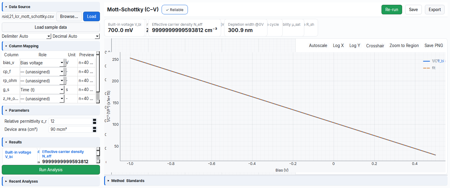
A1 — Mott–Schottky (C–V) · `lcr_mott_schottky`

🎓 What is it for? — A1 Mott–Schottky (C–V): how many carriers are there?

By looking at how the device's capacitance changes as the voltage is varied, this module tells you how much the semiconductor is "doped" (carrier density) and the junction's built-in voltage. Just as the capacitance of a capacitor drops as its plates are moved apart, voltage widens the depletion region, and the slope of this change gives us the density.

Why it's done: It answers the question "how many free carriers per unit volume are there in this material?"
What it teaches / measures: Effective carrier density N_eff, built-in voltage V_bi and the depletion width at 0 V.
Where it's used: Diode/solar cell doping level verification and process control.

Purpose: Extracts carrier density N_eff and built-in voltage V_bi from depletion-region C–V data.

Physics and method. In an abrupt junction the depletion capacitance is C_dep = ε·A/W with W = √(2ε(V_bi−V)/(qN)), so the 1/C² quantity is linear in bias:

Formula 1/C² = 2 · (V_bi − V) / (q · ε_r · ε₀ · A² · N)

The engine applies a linear fit (slope m, intercept b) to the 1/C²–V curve:

N_eff = −2 / (q · ε_r · ε₀ · A² · m) → [m⁻³], then ×10⁻⁶ to [cm⁻³]
V_bi = −b/m (x-intercept)
W_d(0 V) = ε_r·ε₀·A / C(0 V) → [m], then ×10⁹ to [nm]

Input columns: bias_v, cp_f. (At least 5 points, all C > 0, finite bias.)

Parameters:

Parameter	Unit	Description	Default
`eps_r`	—	Relative permittivity ε_r	11.7
`area_cm2`	cm²	Device area	0.09

Outputs:

Key	Unit	Description
`n_eff_cm3`	cm⁻³	Effective carrier density (from slope)
`v_bi_v`	V	Built-in voltage (x-intercept)
`w_d_at_0v_nm`	nm	Depletion width at 0 V
`ms_slope`	1/(F²·V)	1/C²–V slope (< 0 for n-type depletion)
`eps_r_used`	—	ε_r used
`r2`	—	Linear fit goodness

Uncertainty (GUM): u(N)/N = u(m)/|m|; u²(V_bi) = u_b²/m² + b²·u_m²/m⁴ − 2·b·cov(m,b)/m³.

Example file: examples/analysis/21_lcr_mott_schottky.csv — c-Si abrupt junction, f = 10 kHz, bias −1.0…0.5 V (40 points). Expected: N_eff ≈ 1×10¹⁶ cm⁻³ (±2%), V_bi ≈ 0.70 V (±20 mV), W_d(0 V) ≈ 301 nm, r² ≥ 0.98.

N_eff1×10¹⁶cm⁻³

V_bi0.70V

W_d(0 V)301nm

r²≥ 0.98

⚠️

Warning The Mott–Schottky interpretation is valid only in the depletion region where the 1/C²–V slope is negative and linear. If the slope is ≥ 0 the module returns "no linear region found" — review the frequency, bias range and series-resistance roll-off.

Mott–Schottky 1/C-squared–V linear fit plot and carrier density output — **Figure.** The A1 Mott–Schottky module; N_eff and V_bi from the 1/C²–V linear fit.

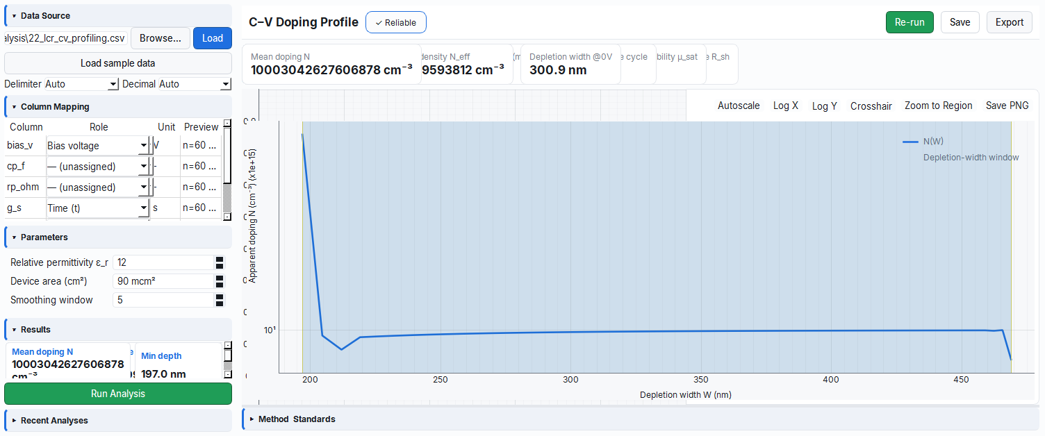
A2 — C–V Doping Profile · `lcr_cv_profiling`

🎓 What is it for? — A2 C–V Doping Profile: how does the density vary with depth?

While A1 gives a single average density, A2 extracts how the doping density varies with depth into the device. Like sounding the bottom of a lake point by point with a plumb line to build a depth map, each voltage corresponds to a depth, and the local density is computed there.

Why it's done: To see whether the doping is uniform or varies with depth.
What it teaches / measures: The depth-resolved N(W) profile, the average density and the depth range covered by the profile.
Where it's used: Doping uniformity quality control and layered-structure analysis.

Purpose: Extracts a depth-resolved (non-uniform) doping profile N(W) from differential C–V.

Physics and method. The differential profiling method:

Formula W(V) = ε_r·ε₀·A / C ; N(W) = C³ / (q · ε_r · ε₀ · A² · |dC/dV|) [m⁻³ → cm⁻³]

The dC/dV derivative is taken first with a Savitzky–Golay (poly = 2) smoothing, then with irregular-spacing-aware numpy.gradient (smoothing window smooth_window). As bias increases W shrinks; as depletion recedes W grows. Only finite, positive points with |dC/dV| > 0 are included in the profile.

Input columns: bias_v, cp_f.

Parameters:

Parameter	Unit	Description	Default
`eps_r`	—	Relative permittivity	11.7
`area_cm2`	cm²	Device area	0.09
`smooth_window`	—	Savitzky–Golay window (odd number)	5

Outputs: n_mean_cm3 (cm⁻³, profile average), n_points_profile (number of valid points), w_min_nm, w_max_nm (nm; the depth range of the profile). Uncertainty: u(N̄) = s/√n (the standard error of the mean of the profile points).

Example file: examples/analysis/22_lcr_cv_profiling.csv — c-Si uniform N(W) ≈ 1×10¹⁶ cm⁻³, bias −1.0…0.4 V (60 points), smooth_window = 5. Expected: the N̄ profile is flat and ~1×10¹⁶ cm⁻³ (2×10¹⁵…5×10¹⁶ band), ≥ 3 valid profile points.

✅

Tip Because the N(W) profile contains C³/|dC/dV| it is very sensitive to noise. For noisy measurements increase the smoothing window (e.g. 7–11), but be careful not to erase real profile features.

Figure. A2 C–V doping profile; the depth-resolved N(W) distribution.

A3 — Impedance (Nyquist) Fit · `lcr_impedance_fit`

🎓 What is it for? — A3 Impedance Fit: modeling the device as a "circuit"

This module fits the impedance measured versus frequency to an equivalent electrical circuit (resistors + capacitor) and finds the values of the circuit elements. Like guessing the circuit inside an unknown box by feeding a signal to its terminals and watching the response, the semicircular (Nyquist) shape of the curve tells us the internal resistances and the capacitance.

Why it's done: To quantify the loss/recombination processes in the device separately.
What it teaches / measures: Series resistance R_s, recombination resistance R_rec, chemical capacitance C_μ and carrier lifetime τ_n.
Where it's used: Solar cell/perovskite device loss analysis and model validation.

Purpose: Applies a complex NLLS fit of an equivalent circuit (Randles type) to the Z–f spectrum; extracts R_s, R_rec, C_μ and carrier lifetime τ_n.

Physics and method. Single-arc Randles circuit:

Formula Z(ω) = R_s + R_rec / (1 + jω·R_rec·C_μ) ; τ_n = R_rec · C_μ ; apex f₀ = 1 / (2π·τ_n)

The circuit is fitted with complex NLLS (modulus weighting 1/|Z|, least_squares TRF, lower bound 0). When the circuit is set to auto it is determined from the device type:

Device type	Default circuit
c_si, iii_v, cigs	`rs_rrec_cmu`
perovskite	`rs_rtr_cgeo_rrec_cmu`
opv	`rs_rrec_cpe`

Supported circuit models:

Circuit ID	Model	Parameters
`rs_rrec_cmu`	R_s–(R_rec‖C_μ)	r_s, r_rec, c_mu
`rs_rrec_cpe`	R_s–(R_rec‖CPE)	r_s, r_rec, cpe_q, cpe_n
`rs_rtr_cgeo_rrec_cmu`	R_s–(R_tr‖C_geo)–(R_rec‖C_μ)	r_s, r_tr, c_geo, r_rec, c_mu
`rs_rrec_cmu_warburg`	R_s–(R_rec‖C_μ)–W	r_s, r_rec, c_mu, warburg_sigma

Input columns: z_re_ohm, z_im_ohm, freq_hz (at least 5 points).

Parameters:

Parameter	Description	Default
`circuit`	Equivalent circuit (auto / 4 models)	auto

Outputs: r_s_ohm (Ω), r_rec_ohm (Ω), c_mu_f (F), tau_n_s (s), chi2, r2, circuit_used (the circuit used). Uncertainty (GUM): u²(τ) = C_μ²·u²(R_rec) + R_rec²·u²(C_μ) + 2·R_rec·C_μ·cov(R_rec,C_μ).

Example file: examples/analysis/23_lcr_impedance_fit.csv — c-Si single-arc, R_s = 5 Ω, R_rec = 5 kΩ, C_μ = 2 nF, 10 Hz–1 MHz (80 points). Expected: R_s ≈ 5 Ω (±5%), R_rec ≈ 5 kΩ (±5%), τ_n ≈ 10 µs (±5%), apex f₀ ≈ 15.9 kHz, circuit_used = rs_rrec_cmu, r² > 0.95.

ℹ️

Note The circuit_used scalar in the output reports which model the auto selection resolved to. Unless you want to fix the circuit manually, auto selects the most appropriate model based on the device type.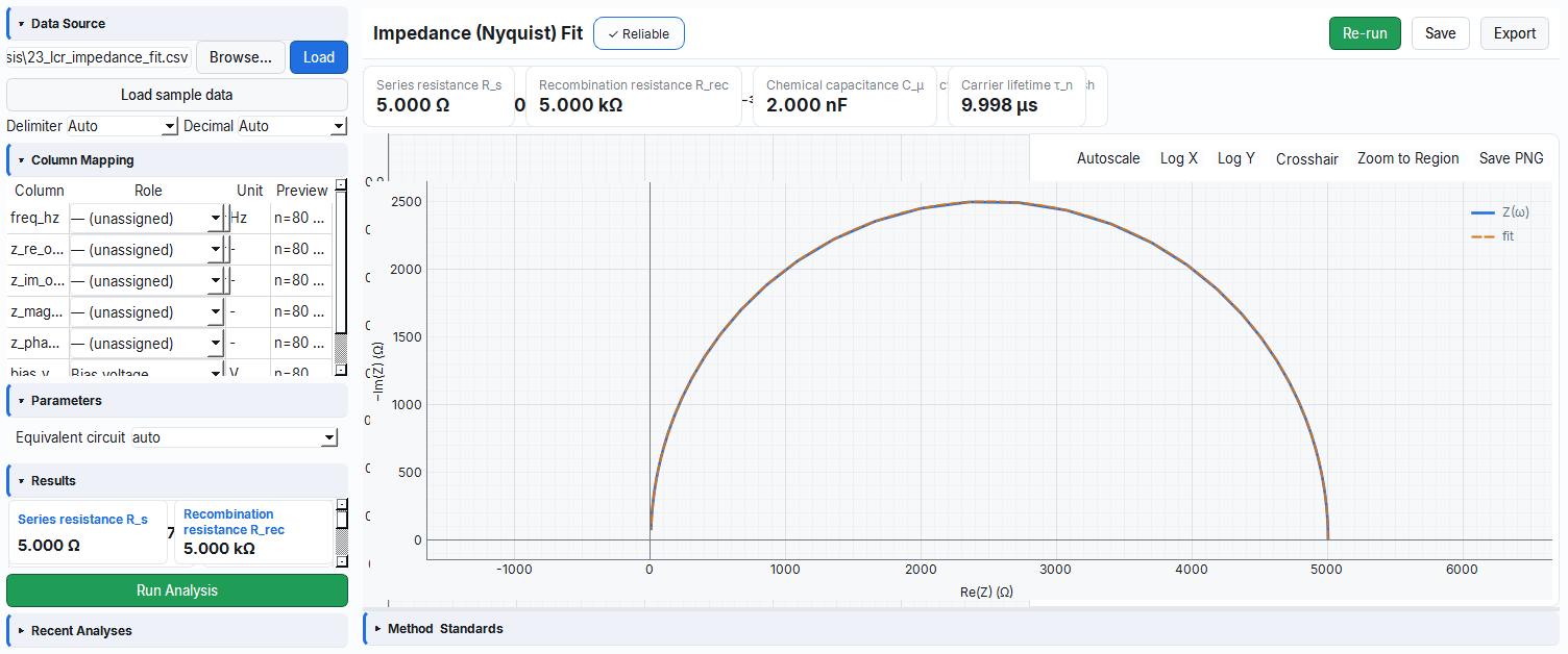

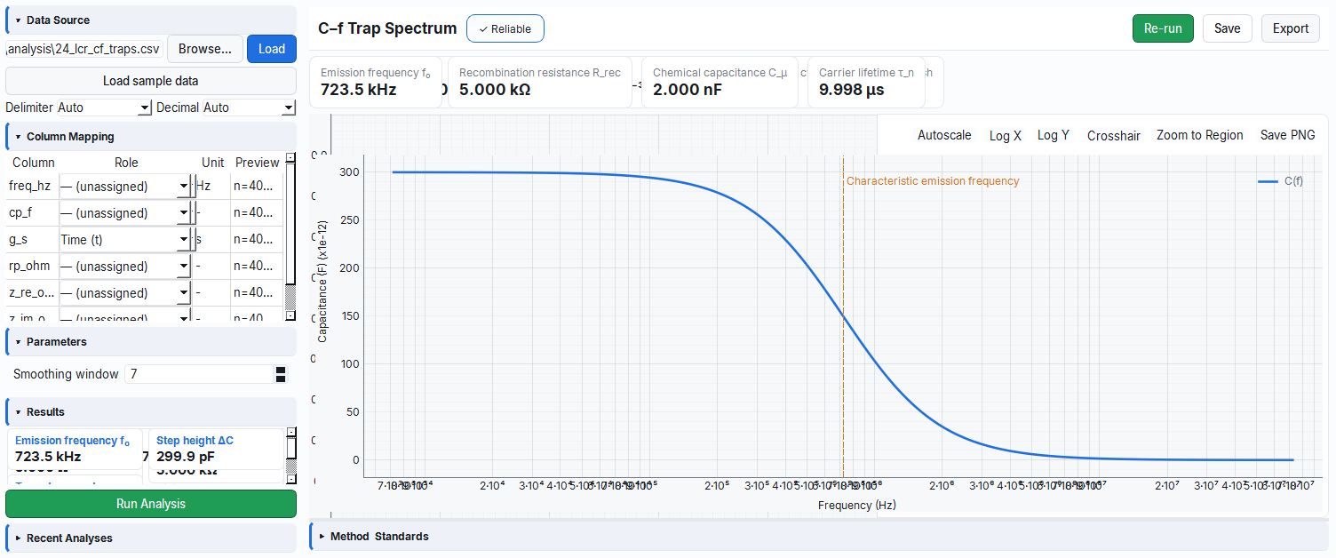
Impedance Nyquist curve and equivalent-circuit fit result — **Figure.** A3 impedance fit; R_s, R_rec, C_μ and τ_n from the Randles single-arc circuit.

A4 — C–f Trap Spectrum · `lcr_cf_traps`

🎓 What is it for? — A4 C–f Trap Spectrum: finding the "clock speed" of defects

Defects (traps) in the material capture and release carriers at a certain rate; this rate corresponds to a characteristic frequency. As the frequency is swept a "step" appears in the capacitance; the module finds the exact frequency of this step. Like turning the dial on a radio until you catch a station, we find the trap's "tuning frequency" by sweeping.

Why it's done: To detect the presence of a trap and the emission frequency that characterizes it.
What it teaches / measures: The threshold emission frequency f₀, the capacitance step height ΔC and the number of detected steps.
Where it's used: Defect screening, material purity and process-induced trap monitoring.

Purpose: Detects the trap steps (Debye relaxation) in the C–f spectrum to find the characteristic (threshold) emission frequency f₀.

Physics and method. For a single Debye trap, C(ω) = ΔC / (1 + (ω/ω_i)²). The −dC/d(ln ω) quantity of this profile peaks at ω = ω_i:

Formula −dC/d(ln ω) = −ω·dC/dω → peak @ ω = ω_i ; f₀ = ω_i / (2π)

The derivative is taken with Savitzky–Golay smoothing; the peak position is determined by parabolic peak refinement (sub-sample precision). The number of steps is counted with scipy.signal.find_peaks (threshold = 20% of the maximum peak).

Input columns: freq_hz, cp_f (at least 6 points, all f > 0).

Parameters: smooth_window (default 7).

Outputs: f0_hz (Hz, threshold emission frequency), delta_c_f (F, capacitance step height = max − min), n_steps (number of detected steps).

Example file: examples/analysis/24_lcr_cf_traps.csv — c-Si single trap E = 0.15 eV, T = 80 K, ν₀ = 1×10¹². Expected: f₀ ≈ 724 kHz (±5%), n_steps = 1, ΔC ≈ 0.3 nF. (2π·f₀ agrees with the emission frequency ω_i = 2ν₀T²exp(−E/kT) to within 5%.)

✅

Tip To see f₀ reliably the sweep band should extend at least two decades below and above the estimated emission frequency (e.g. f₀/100 … 100·f₀). The example is therefore set up log-symmetrically (±2 decades) around f₀.

C–f trap spectrum and emission frequency peak detection — **Figure.** A4 C–f trap spectrum; the threshold emission frequency f₀ from Debye relaxation.

A5 — Trap DOS + Urbach (tDOS) · `lcr_tdos`

🎓 What is it for? — A5 Trap DOS + Urbach: the energy map of defects

While A4 finds a single trap frequency, A5 converts capacitance–frequency data into a defect-density-versus-energy distribution; it also measures the band-edge "blurring" (Urbach energy) if present. Like recording an orchestra and teasing out how many instruments play at each note, it shows how many traps there are at each energy.

Why it's done: To understand whether the defects are at a single energy or in a distribution.
What it teaches / measures: The energy-resolved trap density N_T(E), the peak energy and the Urbach energy E_U (a measure of disorder).
Where it's used: Thin-film disorder/quality assessment (e.g. CIGS, perovskite).

Purpose: Converts C(ω) data into an energy-resolved trap density N_T(E) distribution using the Walter trap-DOS method; extracts the Urbach energy E_U if a band tail is present.

Physics and method. The Walter transform:

Formula E(ω) = k_B·T · ln(ν₀·T² / ω) [eV] ; N_T(E) = −(V_bi / (q·W)) · (dC/dω) · (ω / (k_B·T)) [m⁻³J⁻¹ → cm⁻³eV⁻¹]

dC/dω is taken with a smoothed derivative. The peak energy E_peak and the peak density are determined within N_T(E). In the band-tail region below the peak energy, ln N_T ≈ −E/E_U is linear; the Urbach energy E_U = −1/slope (meV) is computed from the slope.

Input columns: freq_hz, cp_f (at least 6 points).

Parameters:

Parameter	Unit	Description	Default
`nu0`	s⁻¹K⁻²	Attempt frequency ν₀	1×10¹²
`v_bi_v`	V	Built-in voltage	0.7
`w_nm`	nm	Depletion width W	100
`temperature_k`	K	Measurement temperature (must match the generation T)	300
`smooth_window`	—	Smoothing window	7

Outputs: n_t_peak_cm3_ev (cm⁻³eV⁻¹, peak DOS), e_peak_ev (eV, peak energy), e_u_mev (meV, Urbach energy — only if a clean band tail is resolved), r2 (Urbach fit goodness). Uncertainty: u(E_U) = (u_m/m²)·1000.

Example file: examples/analysis/25_lcr_tdos.csv — CIGS, T = 55 K, V_bi = 0.8 V, W = 100 nm, ν₀ = 1×10¹², band tail E_U = 20 meV + traps at 0.10/0.28 eV (emission ~661 kHz). Expected: peak DOS > 0, 0 ≤ E_peak ≤ 0.65 eV, E_U > 0 if present.

⚠️

Warning The temperature_k parameter must equal the temperature at which the measurement was taken; the E(ω) transform depends directly on temperature. If the wrong temperature is entered the energy axis shifts. Because CSV metadata is not carried, verify this value manually.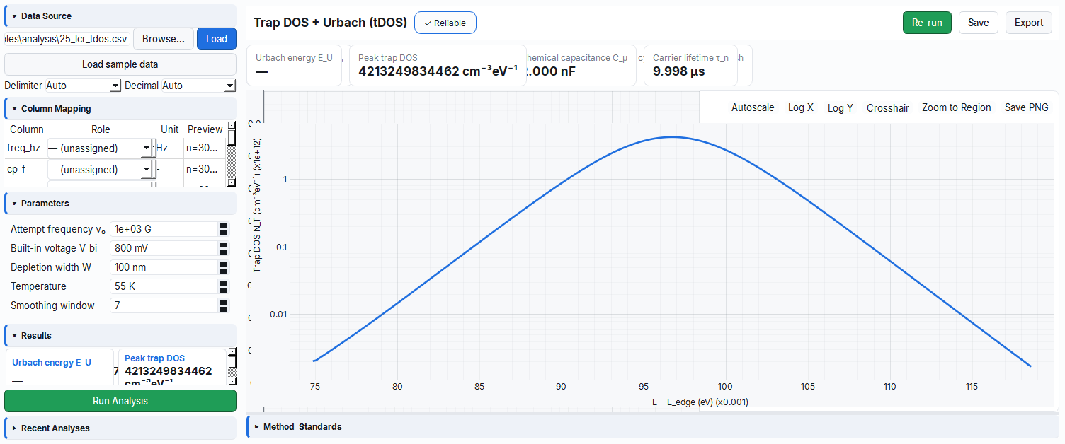

Trap DOS energy distribution and Urbach tail fit plot — **Figure.** A5 trap-DOS (tDOS); the energy-resolved N_T(E) and the Urbach energy.

A6 — Admittance D_it (Conductance Method) · `lcr_admittance_dit`

🎓 What is it for? — A6 Admittance D_it: counting defects at the interface

Electronic states trapped at the interface where two materials meet (e.g. oxide/semiconductor) degrade device performance. This module counts the density of these interface defects from the peak the conductance makes versus frequency. Like counting the mortar cracks between two bricks, it tells you how "clean" the bonding surface is.

Why it's done: To measure interface quality quantitatively and to track process improvement.
What it teaches / measures: The interface trap density D_it and the trap time constant τ_it.
Where it's used: MOS/MIS structures, gate oxide and passivation quality control.

Purpose: Extracts the interface trap density D_it and the trap time constant τ_it using the Nicollian–Brews conductance method.

Physics and method. The parallel conductance quantity G_p/ω:

Formula G_p/ω = ω·G·C_ox² / (G² + ω²·(C_ox − C)²)

This quantity peaks at ω = 1/τ_it. From the peak value:

Formula D_it = (2.5/q) · (G_p/ω)_max / A [cm⁻²eV⁻¹] ; τ_it = 1 / ω_peak ; C_ox = max(C_p) (if no parameter is given)

Input columns: freq_hz, cp_f, g_s (at least 6 points).

Parameters:

Parameter	Unit	Description	Default
`area_cm2`	cm²	Device area	0.09
`cox_f`	F	Oxide capacitance (0 → max C_p is used)	0.0

Outputs: d_it_cm2_ev (cm⁻²eV⁻¹), f_peak_hz (Hz, the G_p/ω peak), tau_it_s (s).

Example file: examples/analysis/26_lcr_admittance_dit.csv — c-Si single interface state (E = 0.15 eV trap, T = 80 K, emission ~724 kHz), A = 0.09 cm². Expected: D_it ∈ [1×10¹⁰, 1×10¹⁴] cm⁻²eV⁻¹, τ_it = 1/(2π·f_peak), f_peak within the sweep band.

ℹ️

Note The 2.5/q prefactor is the standard approximate coefficient of the Nicollian–Brews single-level approximation. If you know C_ox, supply it via the cox_f parameter; otherwise the largest capacitance in the sweep is taken as C_ox.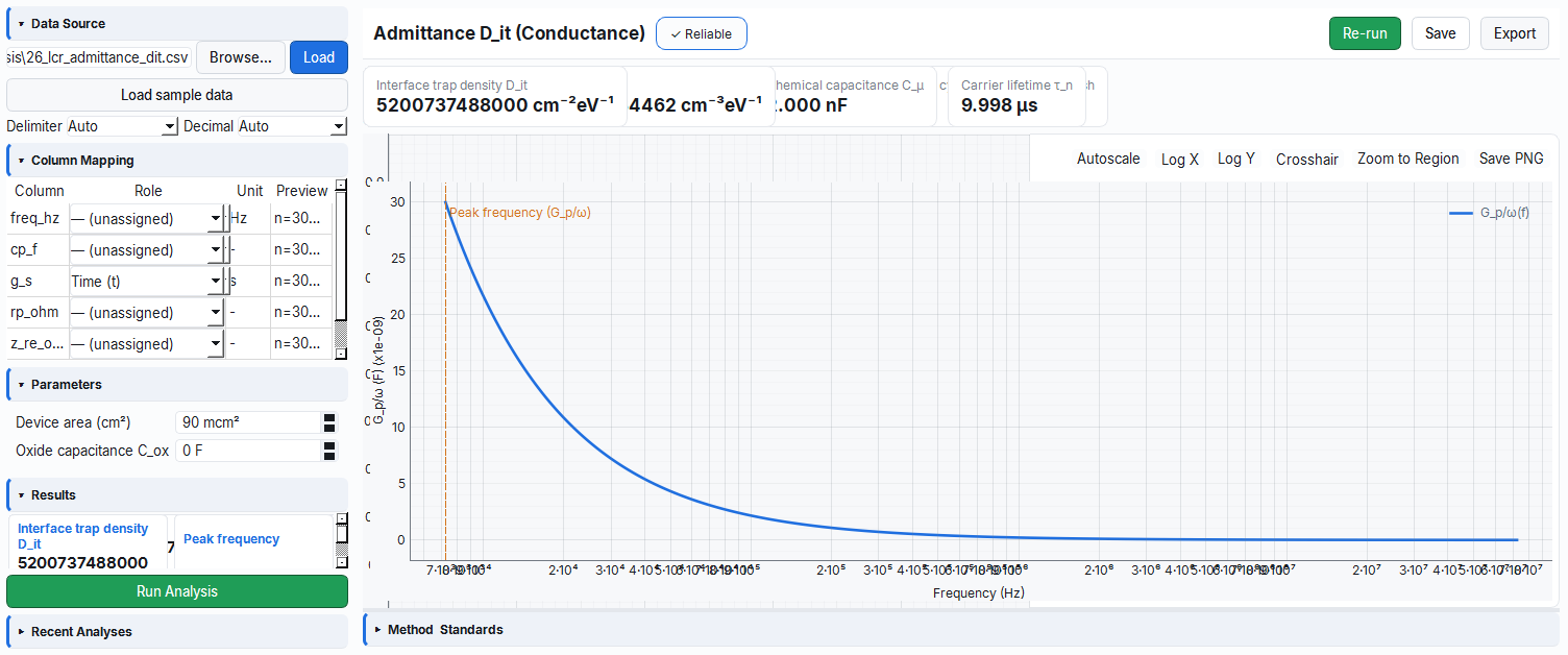

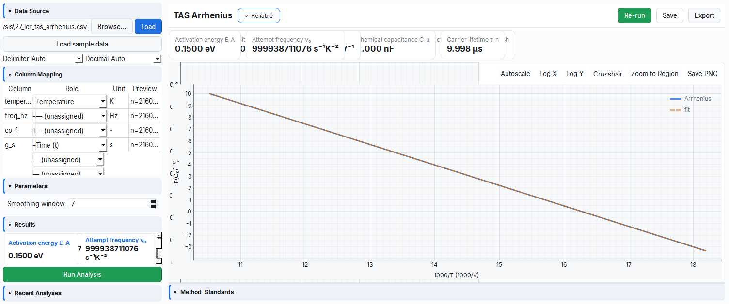
Admittance conductance method Gp/omega peak plot and Dit output — **Figure.** A6 admittance D_it; the interface trap density from the Nicollian–Brews G_p/ω peak.

A7 — TAS Arrhenius · `lcr_tas_arrhenius`

🎓 What is it for? — A7 TAS Arrhenius: extracting the trap's identity via temperature

A trap's emission rate depends very strongly on temperature. This module combines the characteristic frequencies measured at different temperatures to extract the trap's activation energy (its fingerprint). Like computing the "melting energy" of ice by watching how fast it melts at different temperatures, the temperature lever reveals the trap's energy.

Why it's done: To identify a trap by its energy and compare it with the literature.
What it teaches / measures: The trap activation energy E_A and the attempt frequency ν₀.
Where it's used: Deep-level defect identification and material reliability studies.

Purpose: Extracts the trap activation energy E_A and the attempt frequency ν₀ from a temperature-resolved admittance (TAS) stack via Arrhenius analysis.

Physics and method. At each temperature the C–f inflection frequency ω₀(T) is found from the −dC/d(ln ω) peak. An Arrhenius line is then fitted:

Formula ω₀(T) = 2·ν₀·T²·exp(−E_A / (k_B·T)) ; ln(ω₀/T²) = ln(2·ν₀) − E_A/(k_B·T)

Linear fit between ln(ω₀/T²) and 1/T: slope = −E_A/k_B → E_A (eV); intercept → ν₀ = exp(b)/2.

Input columns: temperature_k, freq_hz, cp_f (stack; at least 12 rows, ≥ 5 frequency points at each temperature). At least 4 resolvable temperatures are required.

Parameters: smooth_window (default 7).

Outputs: e_a_ev (eV), nu0_s_k2 (s⁻¹K⁻²), n_temperatures (number of resolved temperatures), r2. Uncertainty: u(E_A) = |u_m|·k_B/q.

Example file: examples/analysis/27_lcr_tas_arrhenius.csv — c-Si single trap, 9 temperatures 55–95 K, 1 Hz–100 MHz sweep. Expected: E_A ≈ 0.15 eV (±10 meV), ν₀ ≈ 1×10¹² s⁻¹K⁻², n_temperatures = 9, r² > 0.95.

✅

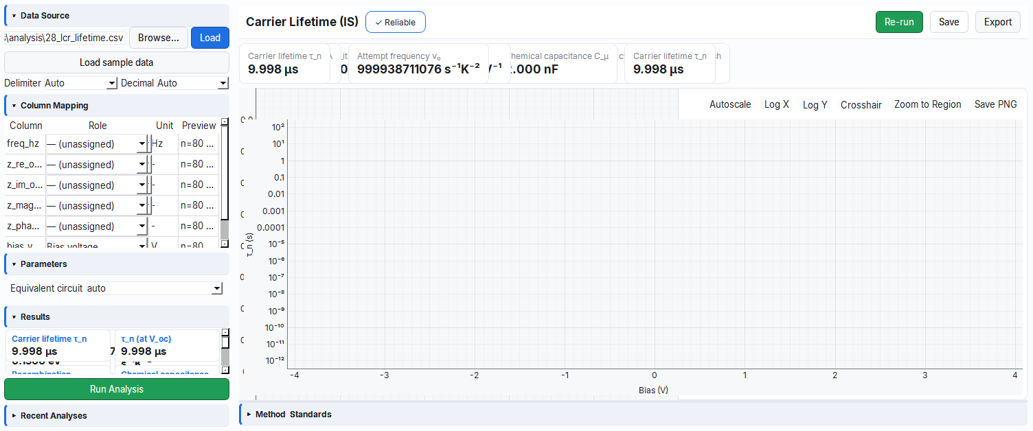
Tip The reliability of the Arrhenius line improves with temperature leverage. A clear C–f inflection frequency should be measured at at least 4–5 temperatures, and the emission frequencies should stay within the device band at every temperature.

TAS Arrhenius line and activation energy fit plot — **Figure.** A7 TAS Arrhenius; the activation energy E_A from the ln(ω₀/T²)–1/T line.

A8 — Carrier Lifetime (IS) · `lcr_lifetime`

🎓 What is it for? — A8 Carrier Lifetime: how long does a carrier live?

From the resistance and capacitance in the impedance fit, this module computes how long, on average, a carrier "lives" before recombining. Like finding the average time people stay in a room from the entry–exit rate, a long lifetime usually means a more efficient device.

Why it's done: To measure the recombination losses that limit device efficiency.
What it teaches / measures: The recombination carrier lifetime τ_n = R_rec·C_μ.
Where it's used: Solar cell efficiency diagnostics and material quality comparison.

Purpose: Extracts the recombination carrier lifetime τ_n = R_rec·C_μ using the Bisquert impedance spectroscopy (IS) interpretation.

Physics and method. Reuses the same circuit fit as A3 in read-only mode (single-source principle):

Formula τ_n = R_rec · C_μ

The uncertainty is computed with the same GUM propagation as A3. For single-condition (single bias/illumination) data the recombination order is not extracted (recombination_order = None; an injection/bias series is needed for the order) and τ_n(V_oc) = τ_n is taken.

Input columns: z_re_ohm, z_im_ohm, freq_hz.

Parameters: circuit (default auto; same options as A3).

Outputs: tau_n_s (s), tau_n_at_voc_s (s), r_rec_ohm (Ω), c_mu_f (F), recombination_order (None for single condition).

Example file: examples/analysis/28_lcr_lifetime.csv — c-Si, R_rec = 5 kΩ, C_μ = 2 nF (same Z–f data as A3). Expected: τ_n ≈ 10 µs (±5%), R_rec ≈ 5 kΩ, C_μ ≈ 2 nF (±10%), recombination_order = None.

ℹ️

Note A single point is not enough to determine the recombination order (e.g. linear/surface vs. Auger); measure a τ_n(V) series at different injection levels. This version provides the single-condition lifetime and leaves the series analysis to a later stage.

Carrier lifetime impedance spectroscopy output — **Figure.** A8 carrier lifetime; τ_n by reusing the A3 circuit fit.

RPS / RUS Family (29–35)

🎓 What is it for? — The RPS / RUS family: measuring a material by "ringing" it

This family vibrates a sample (drives it into resonance) and listens to its natural "ringing" frequencies. Just as the sound a glass makes when you tap it depends on its pitch, size and material, a sample's resonances reveal its stiffness (elastic modulus), piezoelectric response and internal friction.

Why it's done: To measure the material's mechanical/elastic and piezoelectric properties non-destructively.
What it teaches / measures: Resonance frequency, quality factor Q, acoustic attenuation, relative d₃₃, elastic modulus and the full elastic tensor C_ij.
Where it's used: Piezoelectric/ceramic material characterization, phase-transition studies and elastic-constant determination.

The RPS/RUS family reads a lock-in measurement file (harmonic, frequency, X/Y phase, R = |V| amplitude, set temperature) to extract resonance and elastic parameters. The data is grouped by the (harmonic, t_set_k) pair; each group must have at least 5 points.

Basic Lorentzian model (amplitude):

Formula R(f) = R_peak / (1 + ((f − f0)/HWHM)²) ; HWHM = f0 / (2Q) ; FWHM = 2·HWHM = f0 / Q → Q = f0 / FWHM ; area = π · R_peak · HWHM [V·Hz] (full-axis integral of the Lorentzian)

Physical interpretations (Migliori & Sarrao, Resonant Ultrasound Spectroscopy, Wiley 1997; Carpenter et al., EPJB 2003; Salje & Carpenter, J. Phys.: Condens. Matter 2011):

f0² ∝ c_eff/ρ — the square of the resonance frequency is proportional to the effective elastic modulus.
area ∝ d₃₃ — the 1f peak area is proportional to the linear piezoelectric response strength (relative).
FWHM = linewidth ∝ 1/Q — a measure of anelastic loss / domain-wall motion.

⚠️

Warning (Lorentzian vs Fano): This pure-amplitude Lorentzian is a high-Q (Q ≫ 1) approximation. Drive–receive "feedthrough" coupling turns the line shape into an asymmetric Fano profile. If r² < 0.95 an asymmetry_suspect note is added; in this case f0 and area may be biased. For unbiased f0/Q the complex (X/Y) two-pole fit (module 34) is preferred.

⚠️

Warning (area truncation): area = π·R_peak·HWHM is the full-axis integral; it is correct only when the peak fits entirely within the sweep range. The peak's f0 ± 5·HWHM range must stay within [f_start, f_stop]. Otherwise a peak_near_edge / area_truncation_suspect note is added.

29 — RPS Lorentzian Fit · `rps_lorentzian_fit`

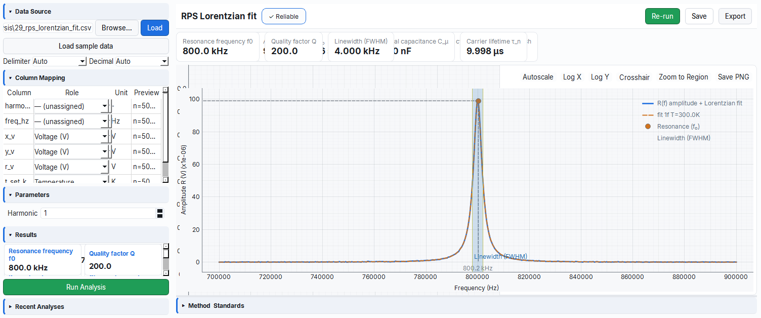
🎓 What is it for? — 29 RPS Lorentzian Fit: measuring a single resonance peak

This module fits a standard bell curve (Lorentzian) to a resonance peak to extract the peak's exact position, sharpness and magnitude. Like measuring exactly what note a guitar string rings at and how "cleanly" it does so, the narrower the peak the less energy the material loses.

Why it's done: To obtain the basic quantities of a resonance reliably and reproducibly.
What it teaches / measures: The resonance frequency f0, the quality factor Q, the peak area and the linewidth (FWHM).
Where it's used: The fundamental building block of all RPS analyses; single-resonance characterization.

Purpose: A Lorentzian fit to the single dominant resonance in each (harmonic, temperature) group; extracts f0, Q, area and linewidth.

Input columns: harmonic, freq_hz, r_v, t_set_k (+ optional x_v, y_v).

Parameters: harmonic (default 1; only the groups of the selected harmonic are fitted).

Outputs (values of the first successful group):

Key	Unit	Description
`f0_hz`	Hz	Resonance frequency
`q`	—	Quality factor Q = f0/FWHM
`area_v_hz`	V·Hz	Peak area = π·R_peak·HWHM
`linewidth_hz`	Hz	FWHM = f0/Q
`chi2`, `r2`	—	Goodness-of-fit metrics
`n_groups_fit`	—	Number of groups fitted

Uncertainties are propagated with GUM: u(Q) includes the cov(f0,HWHM) term; u(area) includes the cov(R_peak,HWHM) term; u(FWHM) = 2·u(HWHM).

Example file: examples/analysis/29_rps_lorentzian_fit.csv — f0 = 800 kHz, Q = 200, R_peak = 1×10⁻⁴ V, single peak @ 300 K. Expected: f0 ≈ 800 kHz (±0.2%), Q ≈ 200 (±5%), FWHM ≈ 4000 Hz (±5%), area ≈ π·10⁻⁴·2000 = 0.6283 V·Hz (±10%), r² > 0.95.

f0800kHz

Q200

FWHM4000Hz

area0.6283V·Hz

RPS Lorentzian resonance peak fit plot — **Figure.** 29 RPS Lorentzian fit; f0, Q, area and linewidth from the single dominant resonance.

30 — RPS Acoustic Attenuation · `rps_attenuation`

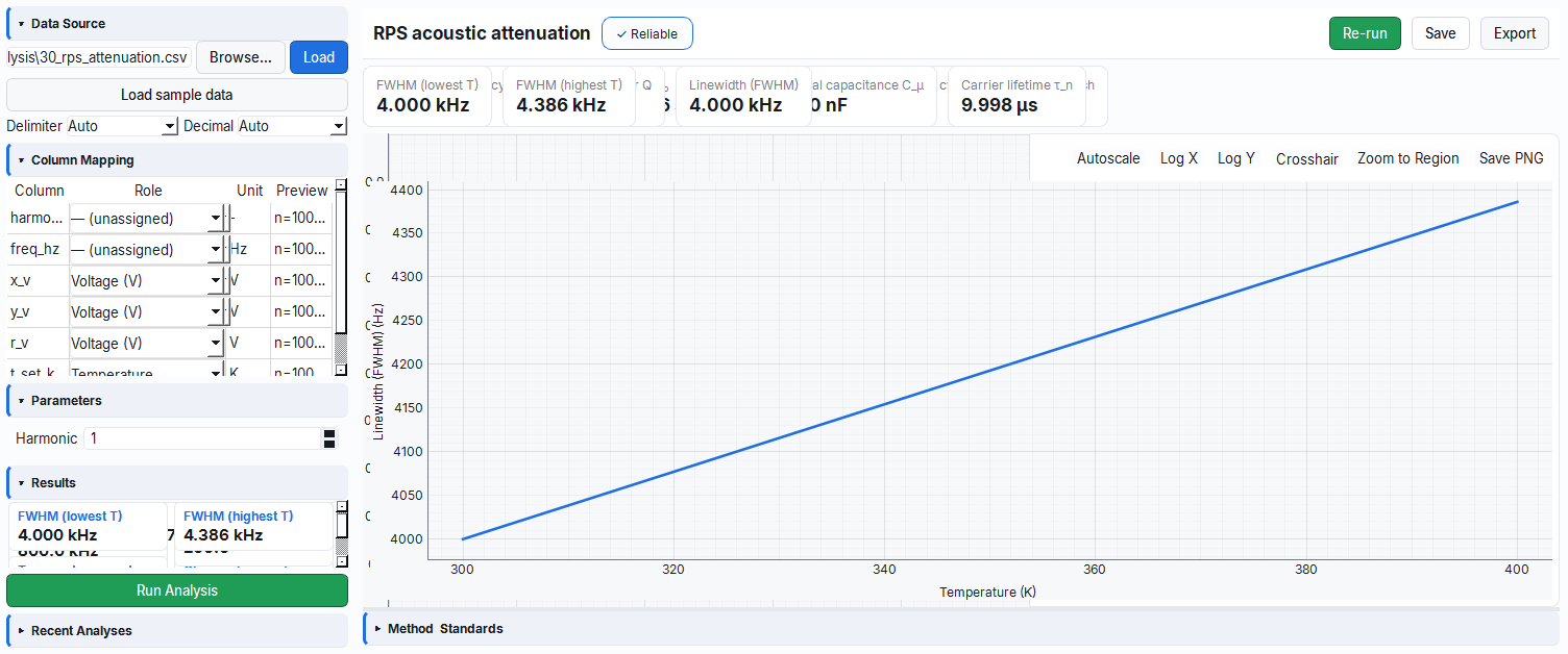
🎓 What is it for? — 30 RPS Acoustic Attenuation: how much energy does the material "absorb"?

This module tracks the material's internal friction (acoustic loss) by watching how much the resonance peak broadens with temperature. Like how quickly the sound of a ringing bell dies away, a broad peak = fast decay = high loss; it produces a pronounced peak at phase transitions.

Why it's done: To detect temperature-dependent loss mechanisms (domain-wall motion, etc.).
What it teaches / measures: The variation of the linewidth (FWHM) with temperature, i.e. the anelastic loss Q⁻¹.
Where it's used: Phase-transition research and attenuation/internal-friction studies.

Purpose: Tracks acoustic attenuation (anelastic loss Q⁻¹) from the variation of the linewidth (FWHM) with temperature.

Physics: Q⁻¹ ∝ FWHM = f0/Q. Mechanisms such as domain-wall motion and point-defect relaxation make the linewidth temperature dependent; it peaks at a phase transition. The module first runs 29 (on the selected harmonic) and extracts the FWHM(T) series from the group results.

Input columns: harmonic, freq_hz, r_v, t_set_k.

Parameters: harmonic (default 1).

Outputs: linewidth_hz_at_min_t (Hz), linewidth_hz_at_max_t (Hz), n_temperatures. The FWHM at each temperature is also returned as an error-barred series.

Example file: examples/analysis/30_rps_attenuation.csv — two 1f groups: 300 K (f0 = 800 kHz, Q = 200 → FWHM = 4000 Hz) and 400 K (f0 = 790 kHz, Q = 180 → FWHM ≈ 4388.9 Hz). Expected: low-T FWHM ≈ 4000 Hz, high-T FWHM ≈ 4389 Hz (both ±5%), n_temperatures = 2; loss increasing with temperature (FWHM_max > FWHM_min).

RPS acoustic attenuation FWHM-temperature series plot — **Figure.** 30 RPS acoustic attenuation; the variation of linewidth with temperature (anelastic loss Q⁻¹).

31 — RPS Relative d₃₃ · `rps_d33_rel`

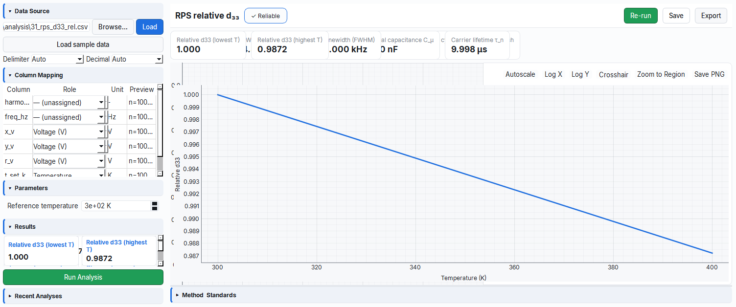
🎓 What is it for? — 31 RPS Relative d₃₃: the variation of the piezoelectric response with temperature

A piezoelectric material produces vibration under voltage; the strength of this response is measured by d₃₃. The module normalizes the area of the fundamental (1f) resonance peak to a reference temperature to track how d₃₃ varies with temperature. Like comparing how "loud" a speaker plays as the temperature changes against a reference.

Why it's done: To see whether the piezoelectric strength weakens near a phase transition.
What it teaches / measures: The relative (normalized) piezoelectric response d33_rel(T); the trend, not the absolute value.
Where it's used: Near-Tc behavior studies in ferroelectric/piezoelectric materials.

Purpose: Tracks the relative piezoelectric response d₃₃ from the variation of the 1f peak area with temperature.

Physics: area_1f(T) ∝ effective d₃₃; d33_rel(T) = area_1f(T) / area_1f(T_ref). Only 1f groups are used. At T_ref the value is 1.000 by definition (its uncertainty is exactly 0).

Input columns: harmonic, freq_hz, r_v, t_set_k. (A 1f fit at at least 2 different temperatures is required.)

Parameters: t_ref_k (reference temperature; default is the lowest T).

Outputs: d33_rel_at_min_t, d33_rel_at_max_t, n_temperatures. Uncertainty (GUM, independent fits, cov = 0): u²(d_r) = (1/area_ref)²·u²(area_T) + (area_T/area_ref²)²·u²(area_ref).

Example file: examples/analysis/31_rps_d33_rel.csv — T_ref = 300 K. 300 K area = π·10⁻⁴·2000 = 0.6283; 400 K area = π·0.9×10⁻⁴·2194.4 = 0.6203. Expected: d33_rel(300 K) = 1.000, d33_rel(400 K) ≈ 0.6203/0.6283 = 0.9873 (±5%), n_temperatures = 2.

⚠️

Warning (relative only): This module produces only relative d₃₃. Absolute d₃₃ [pC/N] requires the sample geometry, electrode area, impedance calibration and the system transfer function; these are out of scope. The results are only for temperature-dependent normalized behavior (softening/loss near Tc).

RPS relative d33 temperature curve plot — **Figure.** 31 RPS relative d₃₃; the normalized variation of the 1f peak area with temperature.

32 — RPS Nonlinearity Ratio · `rps_nonlinearity_ratio`

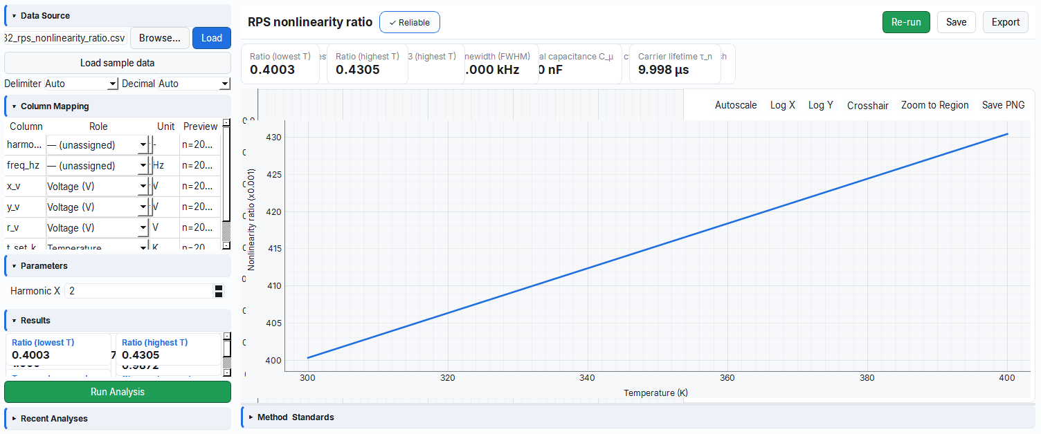
🎓 What is it for? — 32 RPS Nonlinearity Ratio: piezoelectric or electrostrictive?

This module compares the second-harmonic (Xf) peak with the fundamental (1f) peak; the ratio tells you how "nonlinear" the material response is. Like feeding a pure note to a speaker and looking at how much unwanted extra tone appears at the output, it separates the linear piezoelectric contribution from the electrostrictive one.

Why it's done: To separate the linear response that arises from symmetry breaking from the nonlinear response present in every phase.
What it teaches / measures: The Xf/1f peak-area ratio (a measure of nonlinearity) and its variation with temperature.
Where it's used: Ferroelectric phase-transition and symmetry diagnostics.

Purpose: Separates the piezoelectric (1f) and electrostrictive (Xf) responses from the ratio of the even-harmonic (Xf) peak area to the 1f area.

Physics: nonlinearity_ratio(T) = area_Xf(T) / area_1f(T). 1f represents the linear piezoelectric response (requires broken inversion symmetry), Xf the nonlinear / electrostrictive response (allowed even in a centrosymmetric phase) (Carpenter et al., EPJB 2003, Eqs. 4–5).

Input columns: harmonic (1 and Xf), freq_hz, r_v, t_set_k.

Parameters: harmonic_x (the Xf harmonic multiplier; default 2). The module runs separate Lorentzian fits for 1f and Xf and matches the common temperatures.

Outputs: ratio_at_min_t, ratio_at_max_t, n_temperatures. Uncertainty (GUM, independent fits).

Example file: examples/analysis/32_rps_nonlinearity_ratio.csv — 300 K: 1f (R = 1×10⁻⁴, Q = 200) area = 0.6283; 2f (R = 0.3×10⁻⁴, f0 = 800.2 kHz, Q = 150) area = π·0.3×10⁻⁴·2667.3 = 0.2513. Expected: ratio(300 K) ≈ 0.2513/0.6283 = 0.400 (±15%), n_temperatures = 2; 2f < 1f (ratio < 1, slight nonlinearity).

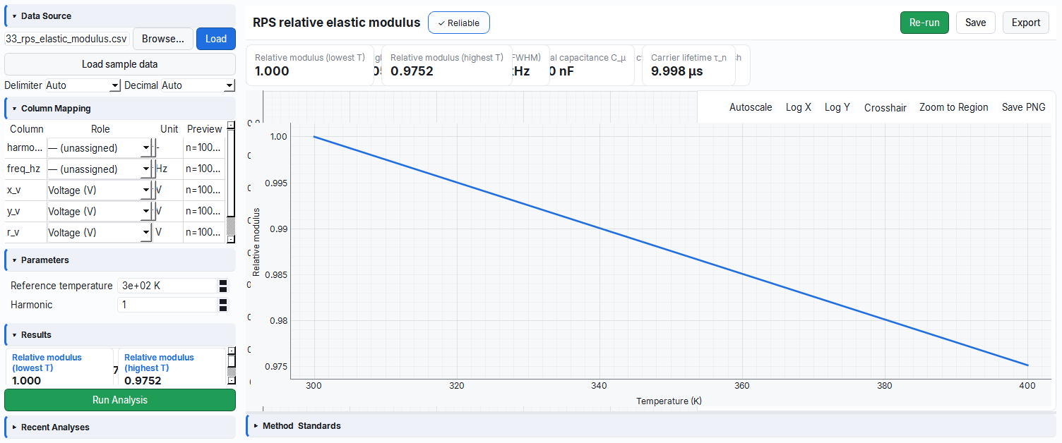
RPS nonlinearity ratio Xf/1f plot — **Figure.** 32 RPS nonlinearity ratio; piezoelectric–electrostrictive separation from the Xf/1f area ratio.

33 — RPS Relative Elastic Modulus · `rps_elastic_modulus`

🎓 What is it for? — 33 RPS Relative Elastic Modulus: the temperature curve of material stiffness

The square of the resonance frequency is proportional to the material's stiffness (elastic modulus). This module tracks the relative stiffness from the variation of f0² with temperature and reveals the "softening" at phase transitions. Like the pitch of a guitar string dropping as it loosens when heated, a drop in pitch indicates the material is softening.

Why it's done: To detect temperature-dependent elastic softening/stiffening and phase transitions.
What it teaches / measures: The relative elastic modulus (f0(T)/f0(T_ref))² and the temperature trend.
Where it's used: Phase-transition/critical-behavior research and thermomechanical characterization of materials.

Purpose: Tracks the relative elastic modulus from the f0²(T)/f0²(T_ref) ratio; reveals the softening at a phase transition.

Physics: Since f0² ∝ c_eff/ρ, modulus_rel(T) = (f0(T)/f0(T_ref))². 1.000 at T_ref.

Input columns: harmonic, freq_hz, r_v, t_set_k. (At least 2 temperatures.)

Parameters: t_ref_k (default is the lowest T), harmonic (default 1).

Outputs: modulus_rel_at_min_t, modulus_rel_at_max_t, n_temperatures, r2_modulus_trend (the goodness of the modulus–T linear trend). Uncertainty (GUM): u²(m_r) = (2f0_T/f0_ref²)²·u²(f0_T) + (2f0_T²/f0_ref³)²·u²(f0_ref).

Example file: examples/analysis/33_rps_elastic_modulus.csv — two 1f groups; f0(400 K)/f0(300 K) = 790/800. Expected: modulus_rel(300 K) = 1.000, modulus_rel(400 K) = (790/800)² = 0.97516 (±1%), n_temperatures = 2; softening at high T (modulus_max-T < modulus_min-T).

ℹ️

Note (density/geometry assumption): The f0² ∝ c_eff/ρ relation assumes ρ(T)/ρ(T_ref) ≈ 1 and that thermal expansion can be neglected. For a wide temperature range or materials with high thermal expansion this approximation may introduce error.

RPS relative elastic modulus temperature curve plot — **Figure.** 33 RPS relative elastic modulus; the (f0(T)/f0(T_ref))² softening curve.

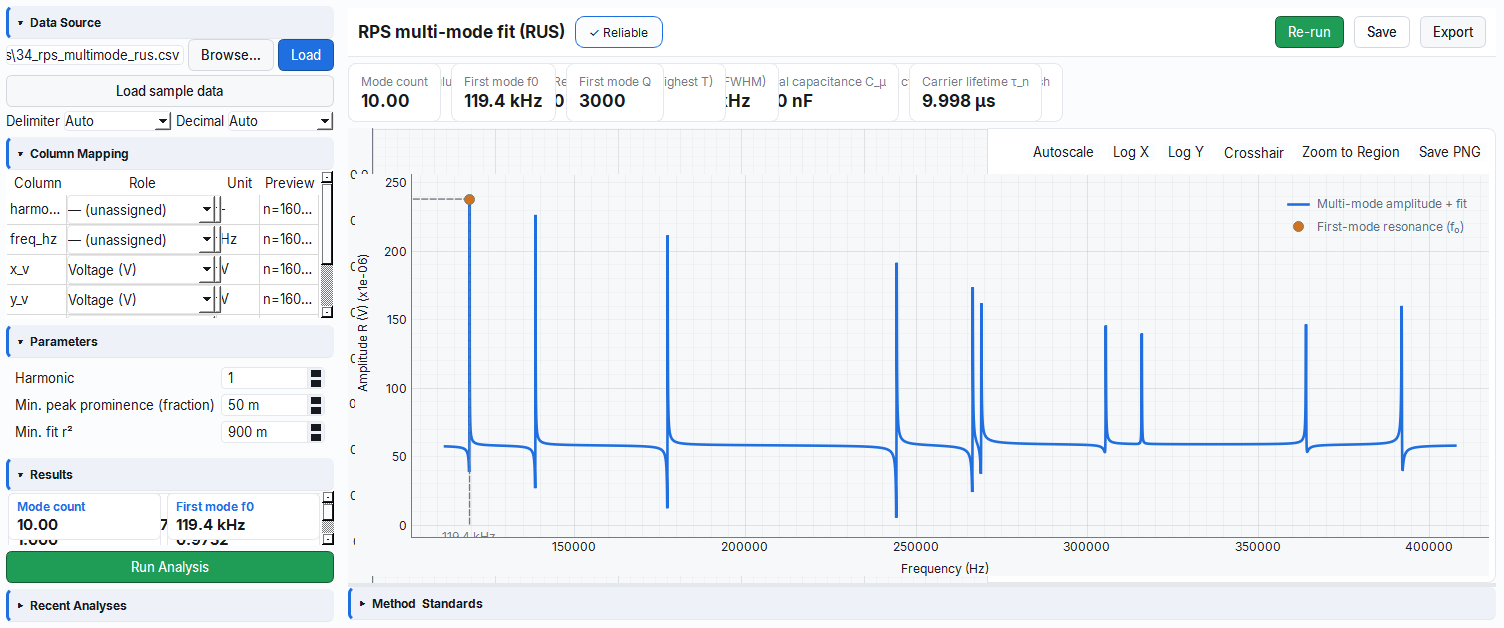
34 — RPS Multi-Mode Fit (RUS) · `rps_multimode_fit`

🎓 What is it for? — 34 RPS Multi-Mode Fit (RUS): capturing all resonances at once

A single sample rings at many different frequencies simultaneously. This module automatically finds all the resonance peaks in the sweep and applies an advanced (complex X/Y) fit to each. Like playing a chord and teasing out each note within it, it prepares the list of modes needed for the subsequent elastic-tensor solution.

Why it's done: To build an accurate and unbiased set of resonances (modes) for the elastic tensor inversion.
What it teaches / measures: The number of modes, the f0/Q/amplitude values of each mode, and the mean Q.
Where it's used: The mode-detection stage of RUS measurements; the preliminary step of the tensor solution.

Purpose: Detects all the resonances in the sweep and applies a complex (X/Y) two-pole fit to each (RUS "Auto-Mark"). Gives unbiased f0, Q, amplitude and linewidth per mode; prepares the measured mode set for the subsequent tensor inversion.

Physics and method. For a single mode, a driven damped harmonic oscillator (normalized complex Lorentzian) + complex background (feedthrough):

Formula L(f; f0, Q) = 1 / (1 + 2i·Q·(f/f0 − 1)) ; V(f) = (b_re + i·b_im) + (a_re + i·a_im)·L(f)

Fitting X and Y jointly removes the feedthrough-induced Fano asymmetry. Peaks are detected with scipy.signal.find_peaks (prominence = a fraction of the R range); each peak is fitted in its own adaptive window; quality gates (r2 ≥ r2_min, q_min ≤ Q ≤ q_max, finite u(f0) ≤ 5%·f0) and mode deduplication are applied.

Input columns: harmonic, freq_hz, x_v, y_v, r_v, t_set_k (≥ 8 points per group).

Parameters:

Parameter	Description	Default
`harmonic`	Restrict to a single harmonic (None → all)	1
`min_prominence_frac`	Min. peak prominence (fraction of R range)	0.05
`r2_min`	Min. complex-fit r² for mode acceptance	0.90

Outputs (summary of the first group): n_modes, f0_first_hz (Hz, the lowest-frequency mode), q_first, mean_q. All mode tables are stored as the mode_groups scalar for the tensor inversion.

Example file: examples/analysis/34_rps_multimode_rus.csv — cubic RPR 2.5 × 5 × 9 mm, ρ = 6000 kg/m³, C11 = 200, C12 = 110, C44 = 70 GPa, Visscher forward spectrum (order 10), 10 resonances, Q = 3000. Expected: n_modes ∈ [8, 14] (≥ 8 resolved), lowest mode f0 ≈ 119.4 kHz (±0.2%), Q_first ∈ [2000, 4000].

RUS multi-mode complex fit; detected resonance modes plot — **Figure.** 34 RPS multi-mode fit (RUS Auto-Mark); the mode set extracted with the complex X/Y two-pole fit.

35 — RUS Elastic-Tensor Inversion · `rps_elastic_tensor`

🎓 What is it for? — 35 RUS Elastic-Tensor Inversion: a full mechanical identity from the ringing

This module works backward from the measured resonance modes and the sample's dimensions/density to solve for all the independent elastic constants (C_ij) of the material. Like back-calculating from all the tones a bell produces what metal it is made of and how stiff it is, it extracts a complete elastic identity from a single measurement.

Why it's done: To obtain the full elastic tensor and the average moduli from a single small sample.
What it teaches / measures: The independent C_ij constants, the VRH aggregate moduli (K, G, E, ν) and the Zener anisotropy.
Where it's used: Elastic-constant determination in materials science, crystal anisotropy and quality verification.

Purpose: Inverts the measured multi-mode resonance spectrum of a sample with known geometry for the independent elastic constants (C_ij) of the selected crystal symmetry; additionally reports the Voigt–Reuss–Hill aggregate moduli (K, G, E, ν) and the Zener anisotropy. This is the flagship output capability of RUS.

Physics and method. The forward problem is the Rayleigh–Ritz / Visscher eigenvalue problem for a free–free rectangular parallelepiped (RPR) (Γa = ω²Ea; W. M. Visscher et al., JASA 90, 2154, 1991). The inverse problem applies nonlinear least squares on the relative frequency residual to the measured frequencies:

Formula residual_i = w_i · (f_calc,i − f_meas,i) / f_meas,i

The number of independent constants depends on the symmetry:

Symmetry	Independent constants	Count
Isotropic	c11, c12	2
Cubic	c11, c12, c44	3
Hexagonal	c11, c12, c13, c33, c44	5
Tetragonal	c11, c12, c13, c33, c44, c66	6
Orthorhombic	c11, c22, c33, c12, c13, c23, c44, c55, c66	9

The aggregate moduli are computed with the Voigt–Reuss–Hill average (Hill 1952), and the Zener anisotropy with A = 2·C44/(C11 − C12) (meaningful only for cubic/isotropic). Born elastic stability (the positive-definiteness of the Voigt matrix) is checked.

Input columns: harmonic, freq_hz, x_v, y_v, r_v, t_set_k (multi-mode extraction is done first with 34; ≥ as many modes as the number of independent constants are required).

Parameters:

Parameter	Unit	Description	Default
`symmetry`	—	Crystal symmetry (isotropic/cubic/hexagonal/tetragonal/orthorhombic)	cubic
`lx_mm`, `ly_mm`, `lz_mm`	mm	Sample edge lengths	4 / 5 / 6
`density_kg_m3`	kg/m³	Sample density	6000
`harmonic`	—	Harmonic to use	1
`order`	—	Forward-solver order	12
`c11_gpa`…`c66_gpa`	GPa	Initial elastic-constant guesses	150/75/75/150/45/45
`n_modes_use`	—	Number of lowest modes to use (0 = all)	0
`piezoelectric_sample`	—	If 1, adds a "stiffened tensor" warning	1

Outputs: c11_gpa, c12_gpa, c44_gpa (+ c13/c33/c66/c22/c23/c55 depending on symmetry), bulk_K_gpa, shear_G_gpa, young_E_gpa, poisson_nu, anisotropy_A, rms_rel_error, n_modes_fit. The uncertainties (u_Cij) reflect only the random frequency-fit spread; they do not include mode-assignment, truncation and geometry/density errors (a lower bound).

Example file: examples/analysis/35_rps_elastic_tensor_rus.csv — cubic, 2.5 × 5 × 9 mm, ρ = 6000, 12 modes; true C11 = 200, C12 = 110, C44 = 70 GPa; off-truth initial guess 180/120/62 GPa. Expected: C11 ≈ 200 (±5%), C12 ≈ 110 (±8%), C44 ≈ 70 (±5%), Zener A = 2·70/(200−110) = 1.556 (±10%), rms_rel_error < 1%. VRH aggregate: K ≈ 140, G ≈ 58.6, E ≈ 154.4 GPa, ν ≈ 0.316.

C11200GPa

C12110GPa

C4470GPa

Zener A1.556

K140GPa

G58.6GPa

E154.4GPa

ν0.316

⚠️

Warning (piezoelectric sample): The forward model is the pure-elastic RPR eigenvalue problem. In a piezoelectric sample the resonances are piezoelectrically stiffened; in this case the result is the stiffened effective tensor, not the true elastic tensor. When piezoelectric_sample = 1 this warning is added automatically. For absolute C_ij use a passive/mechanically-driven sample.

⛔

Danger (reliability): The result is considered ✓ Reliable only if the fit converged and the tensor is positive-definite. Otherwise the module returns analysis_resolved = False and flags the values as "PROVISIONAL — must not be used"; review the initial guess, the number of modes and the solver order. Take into account the assignment_suspect (suspected mode assignment) and truncation_not_converged (insufficient order) notes.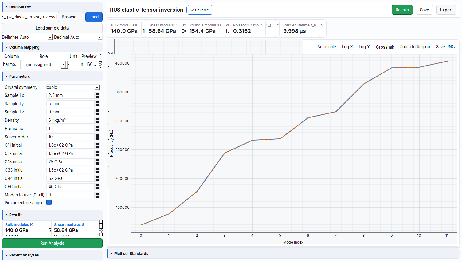

RUS elastic tensor inversion Cij output and aggregate moduli — **Figure.** 35 RUS elastic-tensor inversion; the independent C_ij constants and the VRH aggregate moduli.

Troubleshooting and Tips

Symptom	Possible cause	Solution
Module returned "insufficient data"	Column names differ from expected / too few points	Verify the CSV headers (e.g. `bias_v`, `cp_f`, `freq_hz`, `harmonic`, `r_v`, `t_set_k`); ensure the minimum point counts
Impedance/RPS fit failed (`analysis_resolved = False`)	SciPy is not installed or it did not converge	Install SciPy; review the initial guesses / circuit selection
f0 or E_A far from expected	Measurement temperature entered incorrectly (tDOS/CF/TAS)	Measure at a temperature that brings trap emission into the device band; match `temperature_k` to the measurement value
Trap step not visible	Sweep band does not cover the emission frequency	Do a log sweep of at least ±2 decades around f₀
RPS area/d₃₃ biased	Peak near the sweep edge (`peak_near_edge`)	Widen the sweep to include f0 ± 5·HWHM
Elastic tensor "unreliable" ✕	Insufficient modes / poor initial guess / low order	Try a wider frequency sweep, a lower prominence threshold, a higher `order` and an initial C_ij close to the truth

✅

Tip All LCR/RPS modules are deterministic: the same file and parameters produce the same result. Before adding an analysis to a report, check r2/rms_rel_error and the relevant warning notes; these are the primary indicators of output reliability.

LCR/Impedance and RPS/RUS Analyses

Common Concepts

Data columns and unit notation

Physical constants (CODATA 2019, SI)

Uncertainty and goodness-of-fit metrics

LCR / Impedance Family (A1–A8)

A1 — Mott–Schottky (C–V) · lcr_mott_schottky

A2 — C–V Doping Profile · lcr_cv_profiling

A3 — Impedance (Nyquist) Fit · lcr_impedance_fit

A4 — C–f Trap Spectrum · lcr_cf_traps

A5 — Trap DOS + Urbach (tDOS) · lcr_tdos

A6 — Admittance Dit (Conductance Method) · lcr_admittance_dit

A7 — TAS Arrhenius · lcr_tas_arrhenius

A8 — Carrier Lifetime (IS) · lcr_lifetime

RPS / RUS Family (29–35)

29 — RPS Lorentzian Fit · rps_lorentzian_fit

30 — RPS Acoustic Attenuation · rps_attenuation

31 — RPS Relative d₃₃ · rps_d33_rel

32 — RPS Nonlinearity Ratio · rps_nonlinearity_ratio

33 — RPS Relative Elastic Modulus · rps_elastic_modulus

34 — RPS Multi-Mode Fit (RUS) · rps_multimode_fit

35 — RUS Elastic-Tensor Inversion · rps_elastic_tensor

Troubleshooting and Tips

A1 — Mott–Schottky (C–V) · `lcr_mott_schottky`

A2 — C–V Doping Profile · `lcr_cv_profiling`

A3 — Impedance (Nyquist) Fit · `lcr_impedance_fit`

A4 — C–f Trap Spectrum · `lcr_cf_traps`

A5 — Trap DOS + Urbach (tDOS) · `lcr_tdos`

A6 — Admittance D_it (Conductance Method) · `lcr_admittance_dit`

A7 — TAS Arrhenius · `lcr_tas_arrhenius`

A8 — Carrier Lifetime (IS) · `lcr_lifetime`

29 — RPS Lorentzian Fit · `rps_lorentzian_fit`

30 — RPS Acoustic Attenuation · `rps_attenuation`

31 — RPS Relative d₃₃ · `rps_d33_rel`

32 — RPS Nonlinearity Ratio · `rps_nonlinearity_ratio`

33 — RPS Relative Elastic Modulus · `rps_elastic_modulus`

34 — RPS Multi-Mode Fit (RUS) · `rps_multimode_fit`

35 — RUS Elastic-Tensor Inversion · `rps_elastic_tensor`