Photovoltaic (Solar Cell) Measurements
This chapter covers all measurement modules in the Photovoltaic (PV) family of the Mikrofab measurement software. Every module extracts the J-V (current density vs. voltage) behavior of a solar cell / mini-module / perovskite or silicon test structure using a single-channel SMU (source-measure unit), along with the related stability / aging metrics. All performance metrics are computed through a single pure core, app/analysis/modules/pv.py › compute_pv_metrics, and, for the advanced report, app/analysis/jv_engine.py › analyze_jv_report (Spec v2.0); this way measurement, batch, and the Analysis workspace all return the same numbers (no metric drift).

This chapter explains the ways to measure "how well a solar cell converts light into electricity." You apply a controlled voltage to the cell and read the resulting current that flows; this voltage-current relationship (the J-V curve) reveals the cell's entire character, like the pressure-flow performance report card of a water pump. From it, important properties such as efficiency, stability, and aging are derived.
Physical background: A solar cell is a p-n junction semiconductor that generates electron-hole pairs when light is absorbed; when these pairs are separated by the junction's internal electric field, a photocurrent arises. As external voltage is applied, the junction becomes increasingly forward-biased and a "diode current" eats back into the photocurrent; the characteristic elbowed (knee) shape of the J-V curve arises precisely from the competition between these two currents. Every metric we measure (Voc, Jsc, FF, PCE) summarizes a different aspect of this competition.
- Why it is done: to answer the questions "How well does this cell work, and does it degrade over time?" with numbers.
- What it teaches / measures: fundamental figures of merit such as efficiency (PCE = what percentage of incoming solar power is converted to electricity), open-circuit voltage (Voc = the highest voltage produced when no load is drawn), short-circuit current (Jsc = the light-generated current per unit area), and fill factor (FF = how close the curve is to a rectangle).
- Typical values and interpretation: for single-junction lab cells, Voc ~0.6 V (silicon)–~1.1 V (perovskite), Jsc ~20-40 mA/cm², FF ~0.7-0.8, and PCE ~15-26%; values below these ranges signal losses (high Rs, low Rsh, recombination).
- Common mistakes / cautions: entering the active area or irradiance incorrectly shifts all Jsc/PCE values proportionally; also, looking at a single curve and overlooking hysteresis (the scan-direction effect) leads to a misleading efficiency report.
- Where it is used: in new-material research, perovskite/silicon cell development, quality control, and long-term stability testing.
1. Overview
1.1 Structure of the PV family
The PV modules are grouped under four categories in the sidebar. The table below lists each module's navigation key (nav_key), dispatch mode code, record identifier (measure.pv.*), and screenshot file name.
| Module (sub-heading) | Sidebar name | nav_key | Mode code | Record ID | Screenshot |
|---|---|---|---|---|---|
| Illuminated J-V | Standard / Illuminated J-V | pvws | PV_JV | measure.pv.jv | meas_pvws.png |
| Dark J-V | Dark J-V | pvdarkjv | PV_DARK_JV | measure.pv.dark_jv | meas_pvdarkjv.png |
| Hysteresis J-V | Hysteresis J-V | pvhyst | PV_HYST | measure.pv.hyst | meas_pvhyst.png |
| Pulsed J-V | Pulsed J-V | pvpulsed | PV_PULSED_JV | measure.pv.pulsed_jv | meas_pvpulsed.png |
| Suns-Voc | Suns-Voc | pvsunsvoc | PV_SUNS_VOC | measure.pv.suns_voc | meas_pvsunsvoc.png |
| Intensity Sweep | Intensity Sweep | pvintensity | PV_INTENSITY | measure.pv.intensity | meas_pvintensity.png |
| MPP Tracking | MPP Tracking | pvmpp | PV_MPPT | measure.pv.mppt | meas_pvmpp.png |
| Light Soaking | Light Soaking | pvsoak | PV_SOAK | measure.pv.soak | meas_pvsoak.png |
| Bias Stress | Bias Stress | pvbias | PV_BIAS_DELTA | measure.pv.bias_delta | meas_pvbias.png |
| Degradation | Degradation | pvdegrad | PV_DEGRAD | measure.pv.degrad | meas_pvdegrad.png |
| Thermal Stress | Thermal Stress / Temperature | pvthermal | PV_THERMAL | measure.pv.thermal | meas_pvthermal.png |
| Constant Voltage | Constant Voltage (V) | pvcv | PV_CV | measure.pv.cv | meas_pvcv.png |
| Constant Current | Constant Current (I) | pvci | PV_CI | measure.pv.ci | meas_pvci.png |
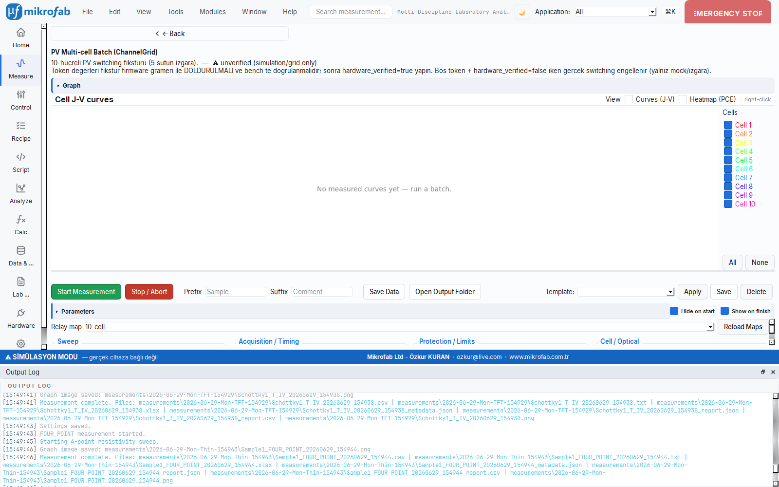
| Multi-cell Batch | PV Multi-cell (ChannelGrid) | pvgrid | — | measure.pv_grid | meas_pvgrid.png |
Grouping:
- J-V Characterization (
navcat.pv_jv): Illuminated / Dark / Hysteresis / Pulsed J-V, Suns-Voc, Intensity Sweep. - Stability & Aging (
navcat.pv_stability): MPP Tracking, Light Soaking, Bias Stress, Degradation, Thermal Stress. - Fixed Point (
navcat.pv_fixed): Constant Voltage (CV), Constant Current (CI). - Photovoltaic / Automation (
navcat.pv_automation): Multi-cell Batch (ChannelGrid).
1.2 Common core concepts
Irradiance is entered manually. In all PV measurements the irradiance value is not read from hardware; the user enters the value manually in the Irradiance (W/m²) field. PCE (efficiency) is computed from this value. The default for Standard Test Conditions (STC, AM1.5G) is 1000 W/m².
0, the input power becomes P_in = 0 and PCE is not computed (the values remain None/"—"). Metrics that are independent of convention, such as Voc, Jsc, and FF, are still reported.Active area (cm²). The cell's active area is required for the current density J = I/A and PCE calculations. The form default is 0.16 cm² (a typical masked lab cell); the actual mask area must always be entered.
Sign convention. In PV devices the sign of the generation current can change depending on the measurement run. There are three options:
| Option | Meaning |
|---|---|
auto | Automatic detection via the power-quadrant integral (S = ∫ V·J dV) (Spec v2.0 §2.1). |
photovoltaic | Current as-is (generation current taken as positive). |
device (dark) | Current is inverted (passive/dark diode convention). |
auto flags the convention as "ambiguous" (ambiguous) and adds a warning to the report. If the result is unexpected, set the convention manually to photovoltaic and measure again.Permissive compliance halt (v3.26). If the current limit (compliance) is reached during a measurement, the software records the point, stops the sweep, and breaks the loop — it never aborts prematurely. This way even a partial curve can be analyzed.
Safe state. At the end of every run (including on error/cancel) the SMU output is brought to a safe value (output OFF) and the mock profile is cleared. In switching (multi-cell) cases the relays are turned off with all_off.
2. Common Parameters
The following fields are common to most PV modules. The columns appear in the measurement window in four logical groups: Sweep · Measurement/Timing · Protection/Limits · Cell/Optics.
| Parameter | Unit | Description | Default |
|---|---|---|---|
device_id | — | Sample / cell identifier (goes into the file name and relay selection). | NUMUNE |
channel | — | Switch matrix channel index (0–47). | 0 |
cell_area_cm2 | cm² | Cell active area (for J and PCE). | 0.16 |
irradiance_w_m2 | W/m² | Manually entered irradiance (AM1.5G = 1000). | 1000 |
convention | — | Sign convention: auto / photovoltaic / device. | auto |
sweep_direction | — | Forward / Reverse / Dual (Dual = hysteresis). | Dual |
voltage_start | V | Sweep start voltage. | -0.2 |
voltage_stop | V | Sweep stop voltage. | 1.2 |
voltage_step | V | Voltage step. | 0.02 |
current_compliance | A | Current limit (compliance). | 1.0 |
nplc | — | Integration time (Number of Power Line Cycles). | 1.0 |
averages | — | Number of averages per point. | 1 |
settling_time_s | s | Wait after setting the voltage. | 0.02 |
measurement_delay_s | s | Extra delay before measurement. | 0.0 |
voltage_limit | V | Source voltage upper limit (protection). | 3.0 |
power_limit | W | Power limit (protection). | 2.0 |
voltage_step must lie within the voltage_start–voltage_stop range; the step cannot be zero (Step sifir olamaz error). Very small step + wide range = long measurement time.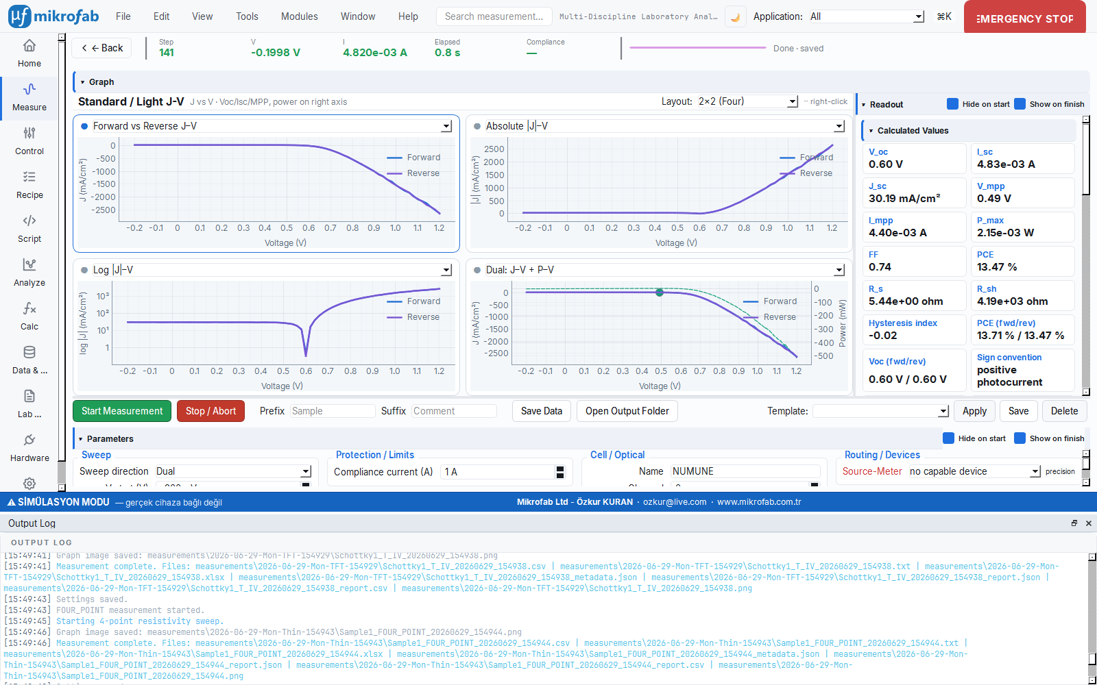
3. Computed Metrics — Single Source
The raw J-V curve on its own is hard to interpret; this module "summarizes" that curve into a few meaningful numbers. Like a report card grade, it converts the cell's performance into standard quantities (Voc, Jsc, FF, PCE) that everyone can compare. Because the entire software produces these numbers from a single core, you see the same result wherever you look.
Physical background: The J-V curve passes through three distinctive points: where the current goes to zero (Voc, the voltage-axis intercept), where the voltage is zero (Isc/Jsc, the current-axis intercept), and the knee point where the power P=V·I peaks (MPP). An ideal cell has a sharp corner (FF→1); the series resistance Rs flattens the slope of the curve near Voc, while the shunt (parallel) resistance Rsh tilts the flat region near V≈0. In other words, the geometry of the curve directly encodes the cell's internal losses.
- Why it is done: it provides a common language for fairly comparing and reporting different cells and measurements.
- What it teaches / measures: Voc = the highest voltage produced when no load is drawn (the lower the recombination, the higher it is); Jsc = the photocurrent collected per unit area (light absorption + carrier collection efficiency); FF = Pmax/(Voc·Isc), the "fullness" of the curve, i.e. the Rs/Rsh quality; PCE = the ratio of output electrical power to incoming light power (%); Rs = contact/conduction series loss (from the slope near Voc); Rsh = leakage/shunt path (from the slope near V≈0).
- Typical values and interpretation: FF>0.75 is excellent, 0.6-0.7 is moderate, <0.5 means high Rs or low Rsh; the area-normalized series resistance (R·A) ~1-3 Ω·cm² is good, >10 Ω·cm² is poor; shunt R·A >1000 Ω·cm² is good, <100 Ω·cm² indicates serious leakage.
- Common mistakes / cautions: a metric that cannot be computed is left as
None(never 0) — mistaking a value for 0 and interpreting it is an error; PCE is not produced when irradiance is 0; the Rs/Rsh fit is unreliable on insufficient data (it falls back to the local-slope method). - Where it is used: at the end of every J-V-based measurement, in the result cards and reports.
All J-V-based modules extract the following metrics for each sweep direction with compute_pv_metrics. A value that cannot be computed is always left as None (never 0); the unit is carried in the field name.
| Metric | Symbol | Unit | Definition / Formula |
|---|---|---|---|
| Open-circuit voltage | Voc | V | The current's persistent first zero crossing (J = 0). |
| Short-circuit current | Isc | A | Current at V = 0 by interpolation. |
| Short-circuit current density | Jsc | mA/cm² | Jsc = Isc · 1000 / A. |
| MPP voltage | Vmpp | V | Power maximum over the [0, Voc] range. |
| MPP current | Impp | A | Current at the MPP. |
| Maximum power | Pmax | W | Pmax = max(V·I) (4000-point fine grid). |
| Fill factor | FF | 0–1 | FF = Pmax / (Voc · Isc). |
| Efficiency | PCE | % | PCE = 100 · Pmax / P_in, P_in = E · A · 10^-4. |
| Series resistance | Rs | Ω | Linear fit over the [Voc, Voc+0.05 V] window. |
| Shunt resistance | Rsh | Ω | Linear fit over the V = 0 ± 0.05 V window. |
Step-by-step calculation flow (input → formula → output):
- Input: the measured
(V, I)pair +A(area),E(irradiance, W/m²), and the convention. - Orientation: the current is converted to
i_genso that the generation current is positive (per the convention). - Voc:
persistent_zero_crossing(V, i_gen)— after the crossing at least 3 points must remain the same sign (noise/S-curve protection; Spec v2.0 §4.2). If not found, it falls back to simple interpolation. - Isc: if
V=0is within range,np.interp(0, V, i_gen); otherwise the point nearest toV≈0. - Jsc:
Isc · 1000 / A→ mA/cm². - MPP: the
[0, Voc]range is interpolated to 4000 points;Pmax, Vmpp, Imppare taken from the maximum ofP = V·I. - FF:
Pmax / (Voc·Isc)→ dimensionless (0–1). It is converted to%on the metric cards. - PCE:
P_in = E · (A · 10^-4)[W];PCE% = 100 · Pmax / P_in. - Rs / Rsh: a linear fit
J = mV + bover the relevant voltage window;R = |1000/m|. If the window is insufficient, it falls back to the local-slope method (1/(dI/dV)).
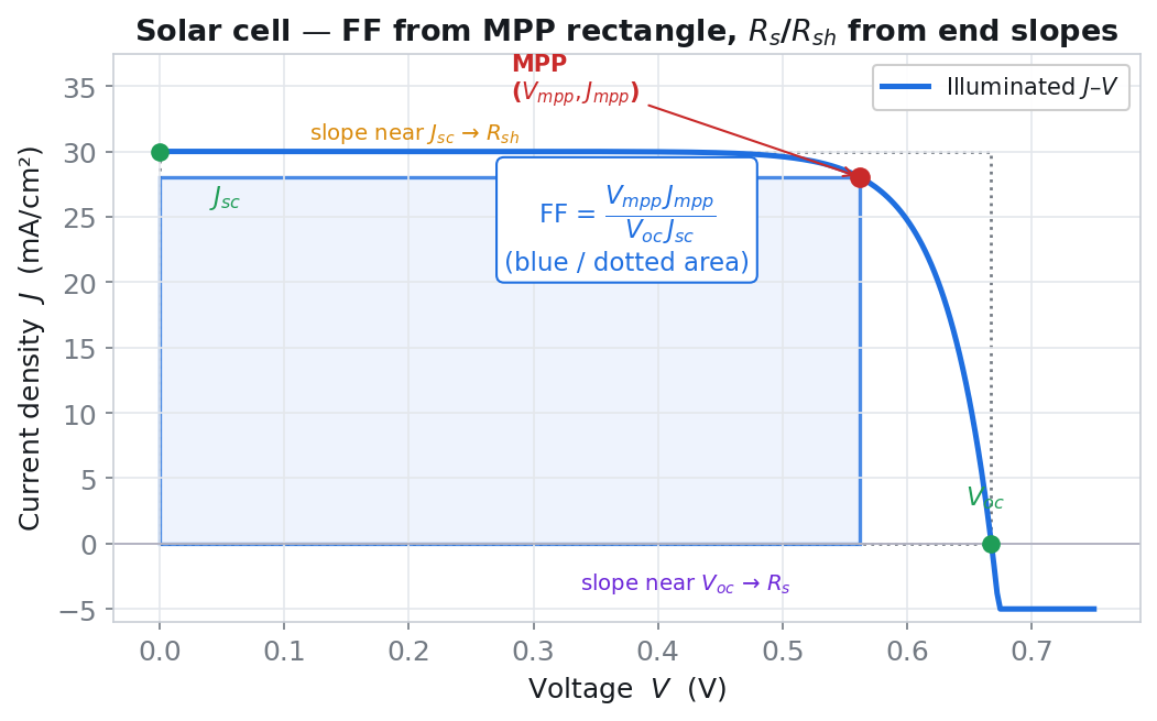
The linear J-V curve (the generation/power region) is used. While Voc is read from the voltage-axis intercept and Isc from the current-axis intercept, FF is derived from the "fullness" of the curve, and Rs and Rsh from the slopes at the two ends.
- FF: the MPP point, where the power (
P = V·I) peaks on the curve, is found; the Vmpp·Impp rectangle formed by projecting this point onto the axes is divided by the Voc·Isc rectangle:FF = (Vmpp·Impp)/(Voc·Isc). - Rs: near Voc (
[Voc, Voc+0.05 V]) a line/tangent is fitted to the steep part of the curve and its slope is taken →Rs = |1000/slope|(the 1000 scaling is because J is in mA/cm²). - Rsh: near short circuit (
V = 0 ± 0.05 V) the slope is taken →Rsh = |1000/slope|; a flat/horizontal region means high Rsh (good), a sloped region means low Rsh (leakage).
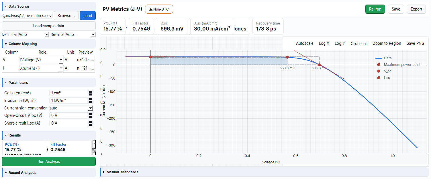
pv_metrics module in the Analysis workspace; it produces Voc/Jsc/FF/PCE from the same core as the measurement.3.1 Hysteresis index (dual direction)
If you scan a cell first in the forward and then in the reverse direction, the two curves do not always overlap; the difference between them is "hysteresis." The hysteresis index reduces this difference to a single number, much like measuring whether a door follows the same path when it opens and when it closes. Close to zero means the cell is stable; large means there are internal dynamics (such as ion migration).
Physical background: The divergence of the forward and reverse scans indicates a slow process inside the cell that responds to voltage with a "lag": migration of mobile ions in perovskites, the filling and emptying of traps at interfaces, or capacitive charge accumulation. Because these slow charges cannot reach equilibrium instantly during the scan, a different current is read at the same voltage in the two directions; the larger the index, the more dominant this slow dynamic.
- Why it is done: to understand whether the measured efficiency is "real" or a misleading artifact that depends on the scan direction.
- What it teaches / measures: HI = (PCErev − PCEfwd)/PCErev, i.e. the relative efficiency difference between the two directions; also the area-based hysteresis Ahyst = the ratio of the area between the two curves to the charge under the reverse-scan curve (a quantity independent of direction choice).
- Typical values and interpretation: HI ≈ 0 is a hysteresis-free, stable device; in good perovskites |HI| < 0.05; HI ~0.1-0.2 indicates pronounced hysteresis; HI > 0.2 indicates strong ion migration / trap filling. In silicon cells HI is typically negligible.
- Common mistakes / cautions: scanning a single direction (only Forward or only Reverse) and never seeing hysteresis; or reporting only the (usually higher) reverse-scan PCE as the "real efficiency." Comparing HI without fixing the scan rate is also misleading — HI is rate-dependent.
- Where it is used: especially in perovskite cells, for reliable efficiency reporting and material stability assessment.
When a Dual scan is performed, the Forward and Reverse directions are summarized separately and the hysteresis index is computed:
Additionally, the pv_hysteresis module in the Analysis workspace also provides an area-based index: the following ratio on a common voltage grid (0..Voc):
HI ≈ 0 means a hysteresis-free, stable device. A positive HI is common in perovskite cells; a large HI is a sign of ion migration / trap filling.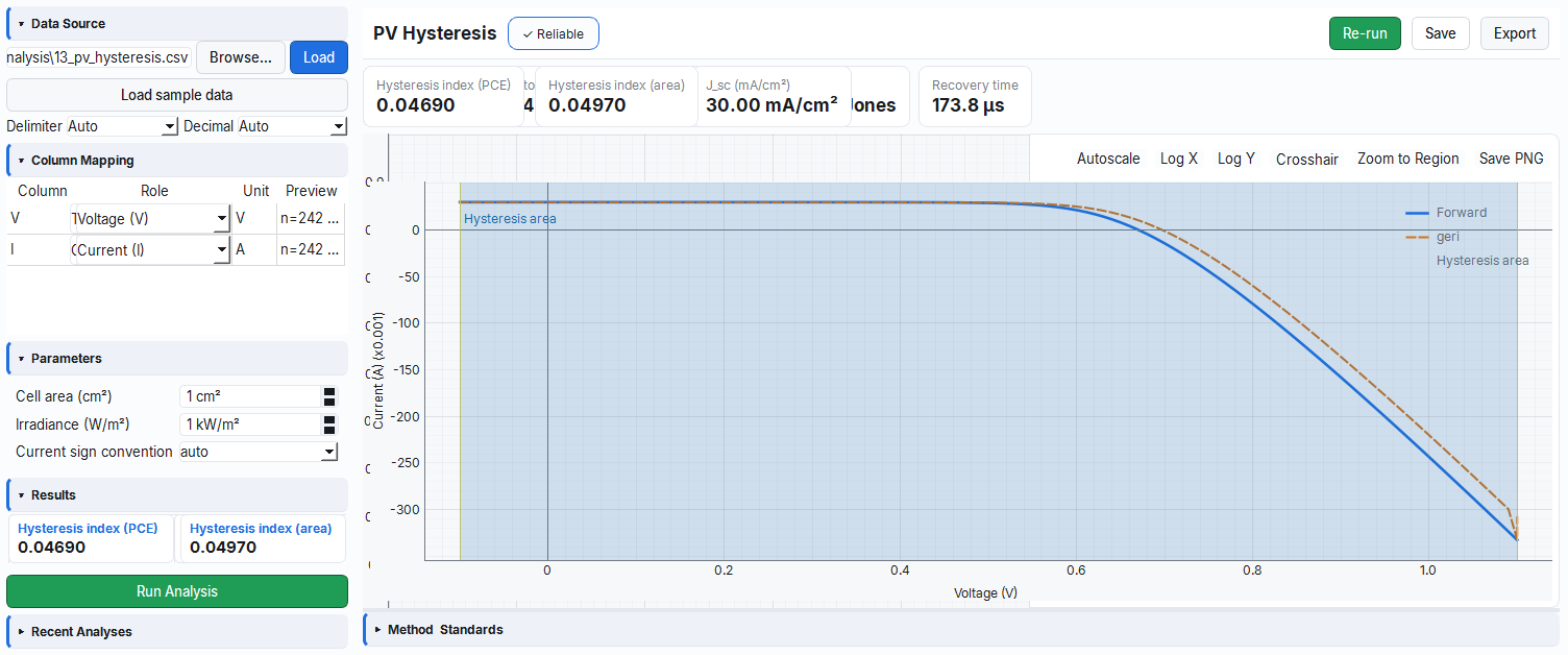
pv_hysteresis analysis module; it reports HIPCE and the area-based hysteresis index together.4. J-V Plot Grid and Metric Cards
Viewing the same measurement with different plot types lets the eye catch different problems; for example, a logarithmic plot brings out small leakage currents while a linear plot emphasizes the overall shape. Like examining a patient with both an X-ray and a blood test, you look at the same data through multiple windows. The metric cards, meanwhile, give a live summary of the most important numbers.
Physical background: The linear J-V shows the overall shape of the curve and the sharpness of the knee (FF); the absolute |J|-V and especially the log|J|-V axis make visible the region where the current changes sign and the leakage/diode currents that are orders of magnitude smaller — the diode region becomes a straight line on the log axis. The dual J-V + P-V pane marks the MPP where power peaks, visually showing the cell's true operating point.
- Why it is done: to quickly inspect the health of the curve by eye during measurement and to spot anomalies (kinks, leakage).
- What it teaches / measures: the linear J-V shape and FF; the leakage/diode region on log|J|-V; in the dual view the point of maximum power (MPP) and live PCE/Voc/Jsc/FF cards (with Δ relative to the previous measurement).
- Typical values and interpretation: on a healthy curve the forward-bias region of log|J|-V is a straight line; a "kink" on the curve (a shoulder/dip before the knee) indicates a barrier or poor contact, and a sloped (non-horizontal) flat region near V≈0 indicates low Rsh (leakage).
- Common mistakes / cautions: forgetting the log axis hides small leakages; overlaying Forward and Reverse in a dual scan and overlooking hysteresis, or misreading the axis range because of autoscaling, are frequent errors.
- Where it is used: in every PV measurement, both for live monitoring and for later exporting plots as PNG.
The PV workspace consists of a configurable 2×2 plot grid (pyqtgraph) and a column of live metric cards. Each pane draws one plot type and all panes are fed from a single central data buffer.
| Plot type | id | Description |
|---|---|---|
| Forward vs Reverse J-V | jv_fr | Linear J-V; Forward and Reverse in separate colors. |
| Absolute |J|-V | jv_abs | Absolute value of the current density. |
| Log |J|-V | jv_log | Y axis logarithmic (diode/leakage region). |
| Dual J-V + P-V | jv_dual | J-V on the left axis, power P-V on the right axis; MPP marked. |
| Time/parameter series | ts | x-y series for MPP, CV, Soaking, Suns-Voc, etc. |
Layout templates: quad (2×2), single, dual_h, dual_v, top1_bottom2, top2_bottom1, left1_right2. Selected from the Layout dropdown in the toolbar; the plot type can be changed from the dropdown in each pane's header. The right-click menu offers: crosshair, autoscale, region zoom, and PNG export.
Axis mapping of the time/parameter modes (the ts pane):
| Mode | X axis | Y axis |
|---|---|---|
| MPP | Time (s) | Power (mW) |
| CV | Time (s) | Current (mA) |
| CI | Time (s) | Voltage (V) |
| BIAS | Time (s) | Current (mA) |
| SOAK / DEGRAD | Time (s) | PCE (%) |
| THERMAL | Temperature (°C) | PCE (%) |
| SUNSVOC | Suns | Voc (V) |
| INTENSITY | Suns | PCE (%) |
Metric cards (right column): PCE (highlighted/hero card, with Δ relative to the previous measurement), Voc, Jsc, FF, Rs · Rsh (on a single card), Hysteresis index. FF is shown converted from a fraction to a percentage, and the resistances are shown in engineering notation (mΩ/Ω/kΩ/MΩ/GΩ).
5. Mock Behavior (Hardware-free Operation)
Mock mode is the software simulating an artificial but realistic solar cell without a real device or cell. Like a flight simulator: you can try out all the measurement steps, learn, and test the software without risking anything. Because the simulated cell behaves according to single-diode physics, the resulting numbers are sensible and instructive.
Physical background: The synthetic curve is generated with the single-diode equivalent-circuit equation: J = Jph − J0·[exp(qV/nkT) − 1] − V/Rsh, corrected with the series resistance Rs. That is, a photocurrent source (Iph), a diode (I0, n), a parallel leakage (Rsh), and a series loss (Rs) represent the same physical elements as in a real cell. Because irradiance changes Iph (Iph ∝ E) and temperature changes the thermal voltage kT/q, the light and temperature sweeps respond realistically.
- Why it is done: to enable training, development, and software verification when no lab hardware is available.
- What it teaches / measures: how each PV mode works and what typical results look like; the profile parameters correspond directly to physics:
Iphphotocurrent (Jsc≈30 mA/cm² at 1 sun),I0diode saturation current,n=1.5 ideality,R_s=1 Ω series loss,R_sh=10 kΩ leakage. - Typical values and interpretation: the results expected with this profile are consistent with a real, mid-quality cell (Jsc≈30 mA/cm², n≈1.5 → moderate recombination, high Rsh/low Rs → good FF); when
illuminated=Falseis selected, Iph is zeroed and only the diode + Rs/Rsh remain (dark J-V). - Common mistakes / cautions: mistaking mock results for real device data; also forgetting that the mock profile is only effective on the mock SMU — on real hardware the profile commands are silently ignored (no-op) and the data comes from the real device.
- Where it is used: training/demos, trying out new features, and rehearsing before connecting to a device.
The application runs in mock mode by default; all PV modules can be tried end-to-end without connecting a real SMU. A solar_cell profile is loaded into the mock SMU, and a synthetic J-V is generated according to the single-diode equivalent circuit:
| Mock parameter | Value | Description |
|---|---|---|
Iph | 0.03 · A (A) | Photocurrent → Jsc ≈ 30 mA/cm² at 1 cm². |
I0 | 1e-9 A | Diode saturation current. |
n | 1.5 | Ideality factor. |
R_s | 1.0 Ω | Series resistance. |
R_sh | 1e4 Ω | Shunt resistance. |
T_K | 300 K | Temperature (stepped in thermal mode). |
noise_scale | 0.01 (J-V) / 0.005 (parametric) | Noise scale. |
The mock physics reflects the following realistically: irradiance (suns) scales the photocurrent (Iph ∝ E); temperature affects the thermal voltage (kT/q) — so the Suns-Voc ideality, intensity linearity, and thermal coefficients come out meaningful. illuminated=False (dark J-V) zeroes the photocurrent; only the diode + Rs/Rsh remain.
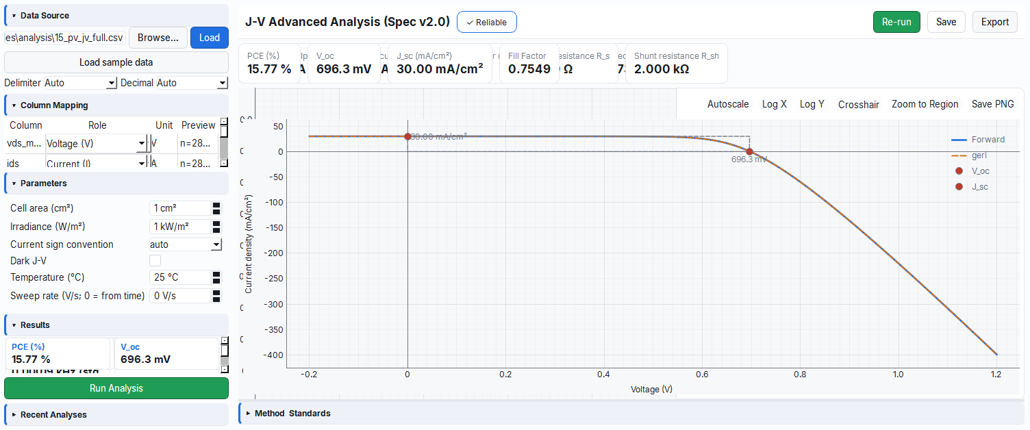
6. Spec v2.0 Advanced J-V Report
The core metrics summarize the cell; the advanced report extracts a much deeper "full blood panel" from the same curve. Think of it like a detailed inspection that reports not just a car's speed but also its engine, brakes, and fuel system. It adds advanced parameters such as fit quality, MPP sharpness, rectification ratio, and, in a dark measurement, the diode ideality.
Physical background: The same (V, J) data reveals different physics when read through different windows: the slope near Voc gives the series resistance (contact/conduction loss), the slope near V≈0 gives the shunt resistance (leakage), the curvature around the knee gives the MPP sharpness (FF quality), and an "S"-bend/kink in the curve indicates a barrier or poor interface that impedes charge extraction. In the dark, the slope of the ln(J)-V line gives the transport mechanism (ideality n) and its intercept gives the saturation current J0.
- Why it is done: to understand not just how well the cell behaves, but why it behaves that way.
- What it teaches / measures: fit quality (R²) = how much the extracted Rs/Rsh can be trusted; MPP sharpness / tolerance window = how flat the power is around the peak (it determines FF); kink/S-curve index = charge-extraction barrier; rectification ratio RR = the diode's forward/reverse current ratio; in the dark, n (conduction mechanism) and J0 (recombination level).
- Typical values and interpretation: good fits have R²>0.99; ideality n≈1 radiative/band-to-band, n≈2 depletion-region (SRH) recombination, n>2 trap/multi-mechanism; a good diode has a rectification ratio of 10³-10⁶; the kink/S-index should be near zero, and if large there is a barrier.
- Common mistakes / cautions: fully trusting Rs/Rsh or n/J0 derived from a low-R² fit; forgetting that in a pulsed measurement the
dynamicblock is skipped (because dV/dt is undefined); when the advanced analysis fails,analysis = Nonebut the core metrics are still valid. - Where it is used: in in-depth research, failure analysis, and device-physics studies.
The measurements in the J-V family (PV_JV, PV_DARK_JV, PV_HYST, PV_PULSED_JV) produce, in addition to the core metrics, a full parameter report (jv_engine.analyze_jv_report, Spec v2.0). This report is carried in the PVJvSummary.analysis field in a JSON-compatible form and is saved to the report/database. Internal units: V [V], J [mA/cm²], P [mW/cm²], R_A [Ω·cm²], C_A [F/cm²], Q_A [C/cm²].
Report blocks:
- metadata: spec version, measurement type (light/dark), active area, light power (mW/cm²), temperature, detected sign convention, scan rate.
- forward / reverse: per direction Voc, Jsc, Vmpp, Pmax, FF, PCE, Rs/Rsh + fit quality (R², number of points, window), MPP tolerance window (P ≥ 0.95·Pmax), MPP sharpness, kink score and S-curve index, rectification ratio (RR), and reverse-bias leakage current.
- hysteresis: ΔJ(V) statistics (max/mean/RMS),
HI_PCEand its symmetric variant, area-based hysteresisA_hyst(power quadrant[0, Voc]), and parameter differences (ΔVoc, ΔJsc, ΔFF, ΔPCE). - dynamic: if time/sweep-rate data is available, the scan rate (V/s), charge density
Q_A, hysteretic chargeQ_hyst, scan energyE_A(net + generated-only), and the apparent capacitanceC_A. In a pulsed measurement (pulsed) this block is skipped (dV/dt undefined). - diode: only in dark J-V — the ideality factor n and the saturation current density J0 (A/cm²) from the
ln(J) = ln(J0) + qV/(nkT)fit.
analysis = None remains and the core metrics (Voc/Jsc/FF/PCE) are still reported.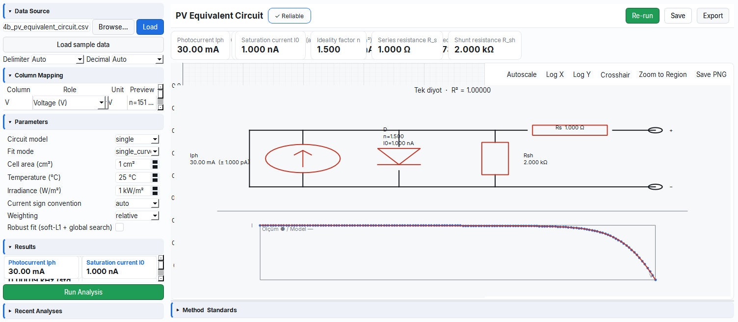
7. Reporting and Automatic Saving
PV measurements are saved automatically. When a run finishes, the DataWriter writes the raw points and the summary to the output folder in the configured export formats (default CSV / TXT / XLSX); the summary is then committed to the database. The Save button opens the last save folder (since PV already saves automatically, it does not write again).
In report generation, for each J-V run the Spec v2.0 advanced J-V report (see §6) is presented together with the summary metrics + plots. For a multi-cell batch, a PCE heatmap and aggregate statistics (mean ± std) are additionally reported.
8. Module Reference
8.1 Illuminated J-V (pvws — measure.pv.jv)
This is the cornerstone of solar cell measurement: it holds the cell under artificial sunlight (a solar simulator), slowly sweeps the voltage, and reads the current. The resulting J-V curve is like the performance report card the cell delivers at full throttle, and the efficiency (PCE) is born here.
Physical background: Under light the cell produces a constant photocurrent; as the voltage increases, the junction becomes forward-biased and the exponentially growing diode current eats back into this photocurrent. That is why the curve is almost flat at low voltage (current ≈ −Jsc) and rapidly enters the knee near Voc: this "knee" is the MPP, where the power is maximum. The sharpness of the knee determines FF, its location determines Voc, and the height of the flat region determines Jsc.
- Why it is done: to answer the question "How efficient is this cell under standard light?"
- What it teaches / measures: Jsc = the light-generated current per unit area; Voc = the highest voltage set by recombination; FF = the fullness of the knee (Rs/Rsh quality); PCE = the ratio of the product of these three to the incoming light power (PCE ∝ Voc·Jsc·FF).
- Typical values and interpretation: for a single-junction cell, Voc ~0.6 V (silicon)–~1.1 V (perovskite), Jsc ~20-40 mA/cm², FF ~0.7-0.8, PCE ~15-26%; FF<0.5 or lower-than-expected Jsc/Voc signals losses (Rs↑, Rsh↓, recombination).
- Common mistakes / cautions: entering the active area/irradiance incorrectly proportionally distorts Jsc and PCE; hitting compliance and clipping the curve gives a wrong Jsc; neglecting the solar simulator's spectrum/intensity calibration (1 sun = 1000 W/m²) shifts the entire efficiency.
- Where it is used: in almost every PV study, it is the first and most frequently performed measurement.
Purpose. A standard J-V sweep under illumination; it extracts Jsc, Voc, FF, and PCE. This is the fundamental measurement of PV characterization.
Input parameters. The common fields in §2 (sweep direction default Dual; irradiance 1000 W/m²; illumination on). Hardware needed: source + meter + light source (solar simulator).
Computed metrics. Voc, Isc, Jsc, Vmpp, Impp, Pmax, FF, PCE, Rs, Rsh; if Dual, additionally the hysteresis index and per-direction PCE/Voc + the full Spec v2.0 report.
Plots. jv_fr, jv_abs, jv_log, jv_dual (MPP marked) — default quad.
Mock. solar_cell profile, illuminated=True, irradiance scales the photocurrent.
8.2 Dark J-V (pvdarkjv — measure.pv.dark_jv)
You turn off the light completely and run the same sweep; with no photocurrent, only the cell's "diode" character remains. Like running an engine with no load and listening to its inner sound, it reveals the cell's internal quality (leakages, ideality).
Physical background: When the photocurrent is zero, the J-V curve returns to a pure diode characteristic: on a semi-logarithmic scale (ln(J)-V) the forward-bias region becomes a straight line. The slope of this line gives the ideality factor n (which mechanism the carriers recombine by), and its vertical intercept gives the saturation current density J0 (the total recombination level). The small current in the reverse-bias region, meanwhile, measures the shunt leakage.
- Why it is done: to see separately the internal losses and diode quality that the light hides.
- What it teaches / measures: ideality n = the conduction/recombination mechanism (1 ideal, 2 depletion-region SRH); J0 = saturation current density, small means low recombination; Rsh = shunt/leakage from the slope near V≈0; rectification ratio = the forward/reverse current ratio (diode quality).
- Typical values and interpretation: n ≈ 1-2 is healthy (n>2 trap/multi-mechanism); the smaller J0 the better (silicon ~10⁻¹²-10⁻⁹ A/cm²); a rectification ratio of 10³-10⁶ is a good diode; a low Rsh (large reverse leakage) indicates a shunt problem.
- Common mistakes / cautions: expecting PV performance metrics (Voc/FF/PCE) in the dark — these are undefined; doing the
ln(J)-Vfit in the wrong (high-bias, series-resistance-dominated) region inflates n; if full darkness is not achieved, the residual photocurrent biases J0. - Where it is used: in diagnosing recombination and leakage sources and in comparing material quality.
Purpose. A J-V sweep without light; it extracts the diode ideality n, saturation current J0, and series/shunt resistance. There is no photocurrent.
Input parameters. The common fields; there is no irradiance field (no light). The convention is usually device (dark). Hardware: source + meter (no light needed).
Computed metrics. Rsh (V≈0 fit), rectification ratio, reverse leakage; the Spec v2.0 diode block: n and J0 from the ln(J)-V fit. PV performance metrics (Voc/FF/PCE) are undefined in the dark.
Plots. In particular jv_log (semi-logarithmic forward bias) is the diagnostic one.
The semi-logarithmic plot of the dark J-V (ln(J)–V, forward-bias region) is used; in this region the curve fits a straight line: ln(J) = ln(J0) + qV/(nkT).
- Step: In the mid forward-bias region (the flat part, outside the Rsh leakage near V≈0 and the high-bias Rs dominance), the slope of the line is taken.
- Step: The same line is carried to
V = 0by extrapolation; the vertical-axis intercept givesln(J0). - Result:
n = q/(kT·slope)(at 300 K,kT/q = 0.025852 V);J0 = exp(intercept)[A/cm²].
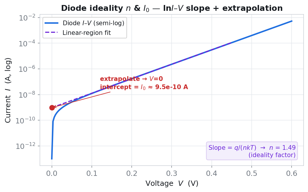
ln(J)–V → ideality n; extrapolating the line to V=0 → saturation current J0.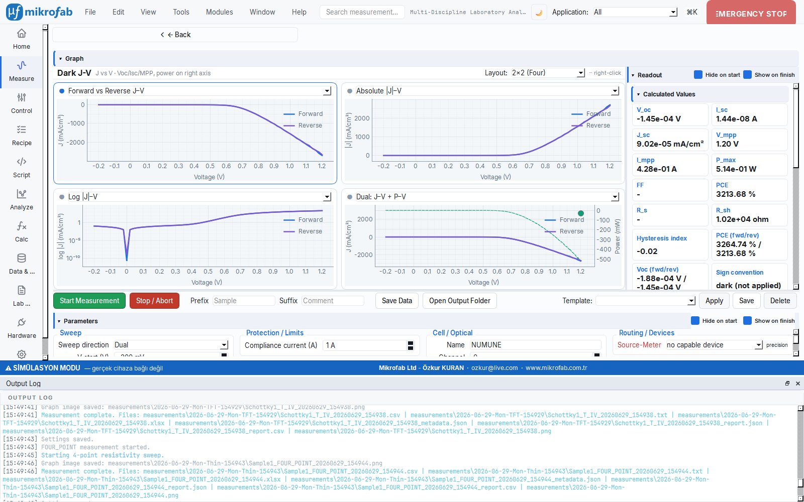
jv_log pane shows the diode/leakage region.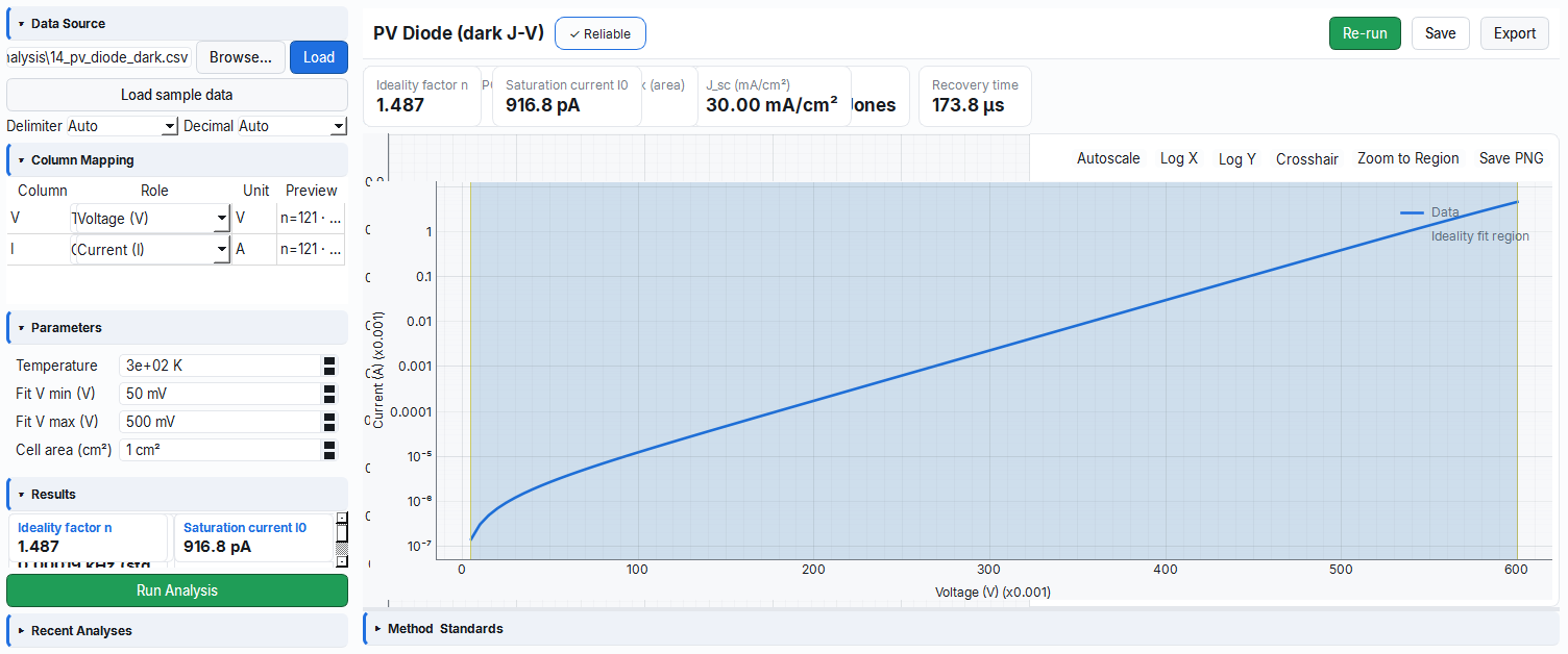
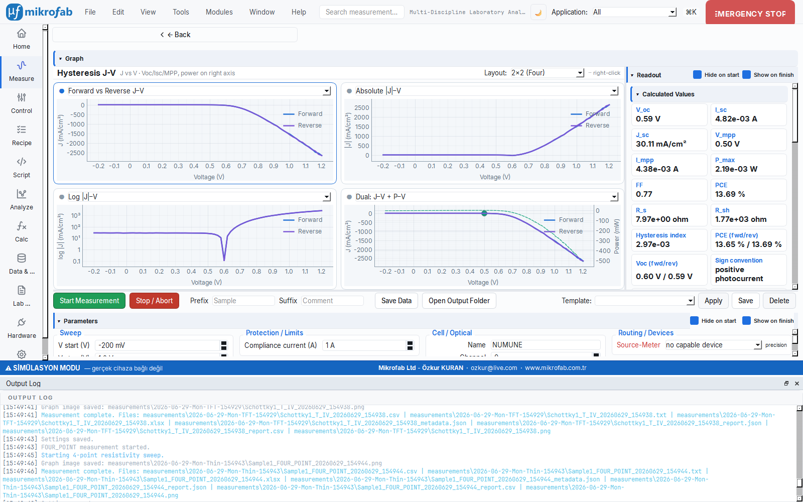
pv_diode analysis module; ideality factor n and saturation current J0 from the ln(J)-V fit.8.3 Hysteresis J-V (pvhyst — measure.pv.hyst)
It scans the cell first in one direction and immediately after in the reverse direction, then compares the two curves. The more the two curves diverge, the more "memory" the cell has; this measurement is designed to deliberately measure that divergence. It is like checking whether a spring follows the same path while being stretched and released.
Physical background: The divergence of the curves in the forward and reverse scans stems from slow processes that respond to voltage with a lag: migration of mobile ions in perovskites, the filling and emptying of interface traps, and capacitive charge. Depending on the scan direction, these slow charges are in a different initial state, so a different current is read at the same voltage. The reverse scan generally gives a higher (optimistic) FF/PCE; the difference between them is the magnitude of the hysteresis.
- Why it is done: to measure the scan-direction-dependent deviation in efficiency and test the reliability of the reported efficiency.
- What it teaches / measures: per-direction Voc/PCE; HI = (PCErev−PCEfwd)/PCErev, the relative difference; Ahyst area-based hysteresis; also the ΔVoc/ΔJsc/ΔFF/ΔPCE direction differences (which show which metric is affected by direction).
- Typical values and interpretation: |HI| < 0.05 is negligible (stable); 0.1-0.2 is pronounced; >0.2 is strong ion migration/traps; in silicon HI ≈ 0 is expected, and a notable HI may indicate a measurement/contact problem.
- Common mistakes / cautions: reporting only the reverse PCE as the "real efficiency"; comparing two devices' HI without fixing the scan rate (settling/delay) — HI is rate-dependent; not recording the preconditioning (pre-light-soaking) state.
- Where it is used: especially in perovskite cells, in ion-migration / trap-dynamics studies.
Purpose. A J-V sweep in the forward + reverse directions (Dual mandatory); it extracts the hysteresis index. It is critical in cells with ion migration / trap dynamics (perovskites).
Input parameters. Sweep direction is always Dual (the form does not show a direction selector in this mode). Hardware: source + meter + light.
Computed metrics. Separate Voc/PCE for Forward and Reverse, HI = (PCE_rev − PCE_fwd)/PCE_rev, and additionally the Spec v2.0 hysteresis block (ΔJ statistics, area-based A_hyst, ΔVoc/ΔJsc/ΔFF/ΔPCE).
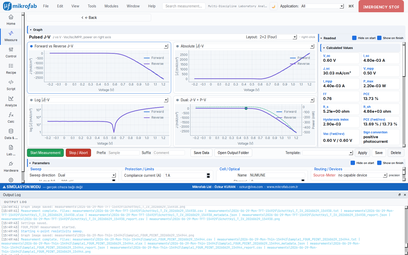
8.4 Pulsed J-V (pvpulsed — measure.pv.pulsed_jv)
Instead of continuously biasing and heating the cell at each voltage point, it applies a short "pulse," measures immediately, and withdraws. Like tapping a hot pan briefly instead of pressing your finger on it continuously, it reduces self-heating and slow transients, thereby capturing the "instantaneous" true behavior.
Physical background: In a continuous sweep, each point both heats the cell and gives the slow charges (ions/traps/capacitance) time to respond to the voltage, distorting the curve with thermal and transient effects. In the pulsed method the cell is mostly held at a neutral baseline voltage, and the measurement is taken only within a short pulse window — if this window is kept shorter than the response time of the slow processes, the measured J-V is largely free of thermal equilibration and transients.
- Why it is done: to obtain a cleaner, transient-free J-V when heating or slow response distorts the curve.
- What it teaches / measures: the standard J-V metrics (Voc, Jsc, FF, PCE), but in a state less affected by transient/thermal effects;
pulse_width_s= the duration of the measurement window (the shorter, the more "instantaneous"),baseline_v= the rest voltage between pulses. - Typical values and interpretation: the pulse width should be shorter than the time constant of the slow processes (typically sub-ms); a large FF/PCE difference between pulsed and continuous J-V indicates that the measured cell is sensitive to thermal/transient effects.
- Common mistakes / cautions: choosing too short a pulse and not leaving the SMU time to settle gives noisy/wrong points; the Spec v2.0
dynamicblock is skipped in pulsed mode (dV/dt undefined) — do not expect capacitance in this block. - Where it is used: for accurate characterization of transient-sensitive or heating cells.
Purpose. It measures each point with a short pulse from a baseline voltage; it reduces self-heating and slow transients. It gives an "instantaneous" J-V for transient-sensitive cells.
Additional parameters.
| Parameter | Unit | Description | Default |
|---|---|---|---|
pulse_width_s | s | Pulse width. | 0.01 |
baseline_v | V | Baseline voltage between pulses. | 0.0 |
Computed metrics. The standard J-V metrics. The Spec v2.0 dynamic block is skipped in pulsed mode (dV/dt undefined). Hardware: source + meter + light.
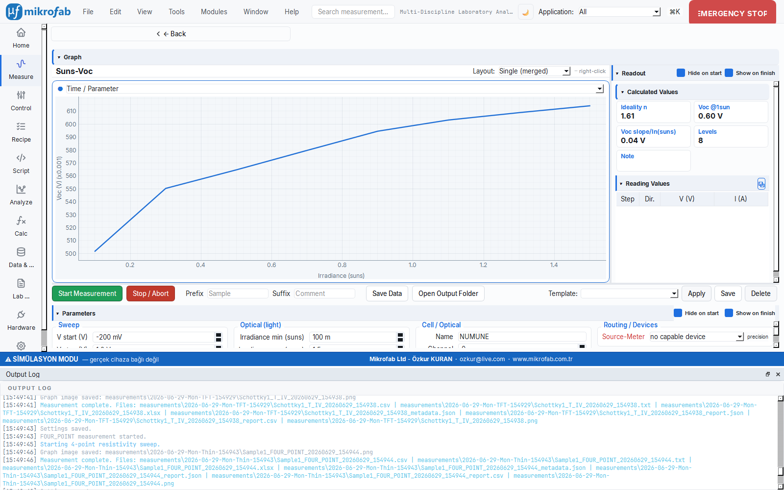
8.5 Suns-Voc (pvsunsvoc — measure.pv.suns_voc)
It varies the light intensity in steps and measures only the open-circuit voltage (Voc) at each level. Because no current flows, the result is unaffected by series resistance; that is why it is like closing the traffic (the current) and measuring the road's true gradient, showing the cell's "raw" quality.
Physical background: At open circuit the net current is zero, so no current passes through the series resistance and Rs has no effect on Voc. Voc is the voltage at which photogeneration and recombination balance, and it increases logarithmically with light intensity: Voc = (nkT/q)·ln(suns) + constant. Therefore, when you plot Voc against ln(suns), the slope directly gives the ideality factor n (the recombination mechanism) and the intercept gives the 1-sun Voc. Comparing the real J-V's FF with this "Rs-free" pseudo-FF separates out the series-resistance loss.
- Why it is done: to reveal the true recombination behavior and ideality that the series resistance hides.
- What it teaches / measures:
ideality_n= the ratio of the Voc–ln(suns) slope to kT/q (recombination mechanism);voc_1sun_v= Voc at 1 sun (intercept);voc_slope_per_ln= the slope; and the Rs-independent pseudo-J-V curve. - Typical values and interpretation: n ≈ 1 low recombination, n ≈ 2 depletion-region (SRH) recombination, n>2 trap/interface dominated; if the pseudo-FF is noticeably higher than the real FF, the difference is the series-resistance loss.
- Common mistakes / cautions: uncalibrated light intensities (suns) distort the slope (n); the fit is unreliable over too narrow a suns range; remember that this n is the depletion-region recombination ideality and is not exactly the same as the J-V "knee" ideality.
- Where it is used: in diagnosing series-resistance losses and in independently verifying cell quality.
Purpose. Voc is measured at varying light intensities (suns); a series-resistance-independent pseudo-J-V and the ideality factor n are extracted.
Additional parameters.
| Parameter | Unit | Description | Default |
|---|---|---|---|
suns_min | suns | Lowest light level. | 0.1 |
suns_max | suns | Highest light level. | 1.5 |
n_levels | — | Number of levels (steps). | 8 |
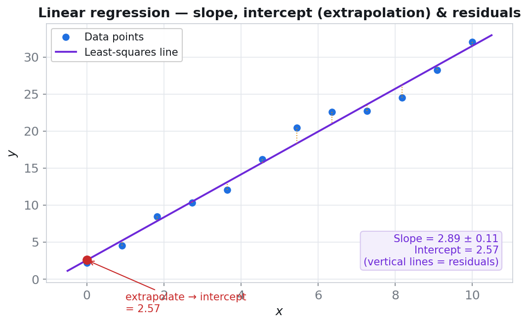
Computed metrics (input → formula → output). At each level Voc is taken from the forward J-V; a linear fit between Voc and ln(suns):
ideality_n      = slope / (kT/q)     ,  kT/q (300 K) = 0.025852 V
voc_1sun_v      = intercept          ,  ln(1) = 0 → Voc(1 sun)
voc_slope_per_ln= slope [V / ln(suns)]The Voc measured at each light level is plotted against ln(suns); the points fit a line, and the slope and intercept of this line are found by least squares.
- Step: A least-squares line fit is performed on the
(ln(suns), Voc)points; the slope =voc_slope_per_ln. - Step: The line is read at the
ln(suns) = 0axis (1 sun) by extrapolation; the intercept =voc_1sun_v. - Result:
ideality_n = slope / (kT/q)(kT/q = 0.025852 V); the fit's residuals (R²) indicate the calibration/noise quality of the light levels.
Hardware: source + meter + light. Plot: ts (suns → Voc).
ln(suns)–Voc slope.8.6 Intensity Sweep (pvintensity — measure.pv.intensity)
It measures a full J-V at different light intensities and extracts how the metrics depend on light. In an ideal cell the current increases in direct proportion to light; like speed increasing proportionally as you press the gas pedal. Deviations from this proportionality reveal losses.
Physical background: The photocurrent is proportional to the number of absorbed photons; therefore, in an ideal cell Jsc increases exactly linearly with the light intensity. If there is trap filling, saturation, or poor carrier collection, this linearity breaks down (Jsc becomes different from expected at low light). Since Voc increases logarithmically with light (~n·60 mV per 10× intensity), PCE generally varies slowly with light intensity.
- Why it is done: to measure whether the cell behaves consistently at low and high light.
- What it teaches / measures:
jsc_linearity_r2= the Jsc–suns linearity quality (R²);jsc_per_sun_ma_cm2= the Jsc slope per sun (photogeneration sensitivity);pce_1sun_pct= the 1-sun efficiency;pce_final_pct= the efficiency of the highest level (the light dependence of PCE). - Typical values and interpretation: jsc_linearity_r2 ≈ 1 (≥0.999) is ideal photocurrent linearity; a low R² indicates traps/recombination or series-resistance-limited collection; PCE dropping at high light says Rs is dominant (loss ∝ I²·Rs), while dropping at low light says Rsh/leakage is dominant.
- Common mistakes / cautions: trusting the suns axis without calibrating the light intensities; interpreting the linearity R² with too few levels (n_levels); hitting compliance at high intensity and clipping Jsc.
- Where it is used: in indoor/low-light performance and in trap/recombination diagnostics.
Purpose. A full J-V at each light level; it extracts the intensity dependence of the metrics (Jsc-suns linearity, PCE(suns)).
Additional parameters. suns_min (0.1), suns_max (1.5), n_levels (8) — same as Suns-Voc.
Computed metrics.
jsc_linearity_r2   = Jsc–suns linear fit quality (R²)
jsc_per_sun_ma_cm2 = Jsc–suns slope  [mA/cm² / sun]
pce_1sun_pct       = PCE at suns=1 by interpolation
pce_final_pct = PCE of the last levelThe Jsc value of each level is plotted against the light intensity (suns); in an ideal cell the points lie on a single line through the origin.
- Step: A least-squares line fit is fitted to the
(suns, Jsc)points; the slope =jsc_per_sun_ma_cm2[mA/cm²/sun]. - Result: the fit quality
jsc_linearity_r2(R²) measures the linearity (≈1 ideal, deviation from a line a sign of loss);pce_1sun_pctis read from the PCE curve by interpolating tosuns = 1.
Hardware: source + meter + light. Plot: ts (suns → PCE).
jsc_linearity_r2 ≈ 1 indicates ideal photocurrent linearity; a low R² is a sign of trap/recombination losses.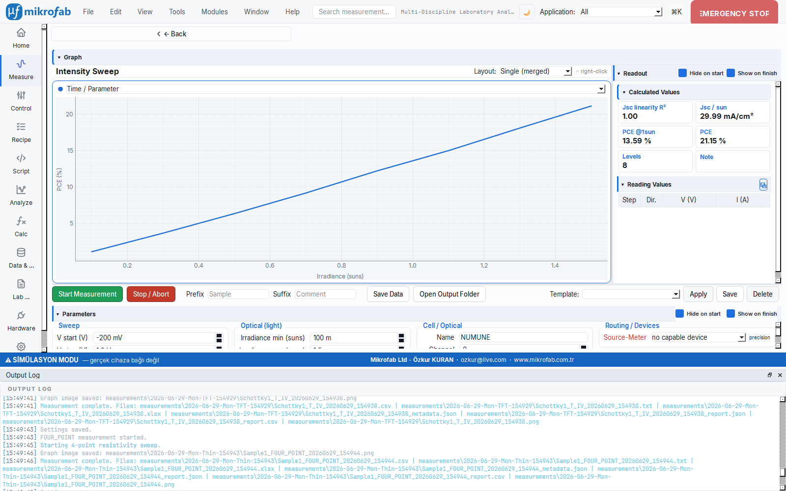
8.7 MPP Tracking (pvmpp — measure.pv.mppt)
It holds the cell at the point where it produces the most power (the maximum power point) and tracks that power over time. The software continuously searches for the best operating point with small trials; like continuously fine-tuning a radio until you find the clearest station. If the power drops over time, the cell is unstable.
Physical background: The variation of power with voltage (P=V·I) peaks at the MPP; on the two sides of this point dP/dV changes sign. The "perturb-and-observe" (P&O) algorithm takes a small voltage step, watches whether the power increases or decreases, and keeps/reverses the step direction accordingly — thus continuously tracking the drifting MPP. Especially in perovskites the power may change with light soaking at the start; the long-term Pmax(t) curve gives the true steady-state efficiency.
- Why it is done: to measure stability under real operating conditions (continuous power draw).
- What it teaches / measures:
pmax_final/best/mean_w= the final/best/mean power over the tracking;vmpp_final_v,impp_final_a= the stable operating point;pce_final_pct= the steady-state efficiency; and the fluctuation/trend (rise = light-soaking improvement, fall = degradation). - Typical values and interpretation: in a stable cell Pmax(t) stays flat/horizontal (steady-state PCE ≈ PCE read from the J-V knee); a continuous decline indicates degradation, a rise then plateau indicates light-soaking improvement; large fluctuation indicates a poorly tuned perturb step or noise.
- Common mistakes / cautions: choosing the start voltage far from Voc so the algorithm reaches the peak late; too large a perturb step causes oscillation around the MPP, too small a step causes slow tracking; keeping the tracking duration shorter than the light-soaking settling gives a misleading (low) steady-state PCE.
- Where it is used: in stability tests and real-use efficiency assessment (especially perovskites).
Purpose. Under constant irradiance, it tracks the maximum power point over time (perturb-and-observe, P&O). It measures the stability of Pmax(t).
Additional parameters.
| Parameter | Unit | Description | Default |
|---|---|---|---|
start_voltage | V | Start voltage (~0.8·Voc). | 0.45 |
voc_hint | V | If >0, start_voltage = 0.8·voc_hint. | 0.0 |
perturb_step_v | V | P&O perturbation step. | 0.01 |
total_duration_s | s | Total tracking duration. | 20.0 |
sample_interval_s | s | Sampling interval. | 0.2 |
Computed metrics. pmax_final/best/mean_w, vmpp_final_v, impp_final_a, pce_final_pct = 100·Pmax_final / (E·A·10^-4), n_samples. Algorithm: if the power increases, continue in the same direction; if it decreases, the direction is reversed. Plot: ts (time → power, mW). Hardware: source + meter + light.
The Pmax(time) curve is used; after the P&O algorithm locks onto the MPP, the curve settles into a horizontal plateau.
- Step: The initial transient region is skipped; the final region where the plateau has flattened is read (
pmax_final_w; the highest point over the tracking ispmax_best_w). - Result:
pce_final_pct = 100·Pmax_final / (E·A·10^-4); a continuously declining plateau means degradation, a plateau that rises then settles means light-soaking improvement.
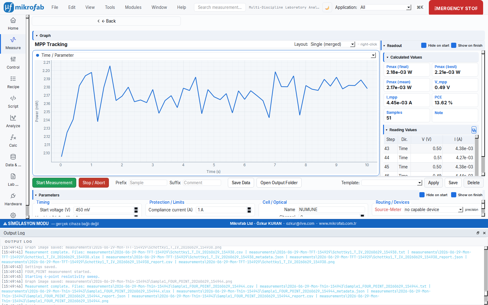
Pmax(t) with the P&O algorithm.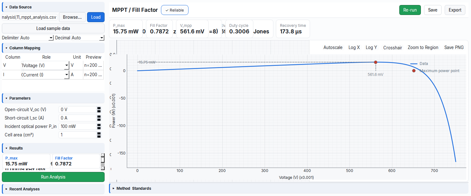
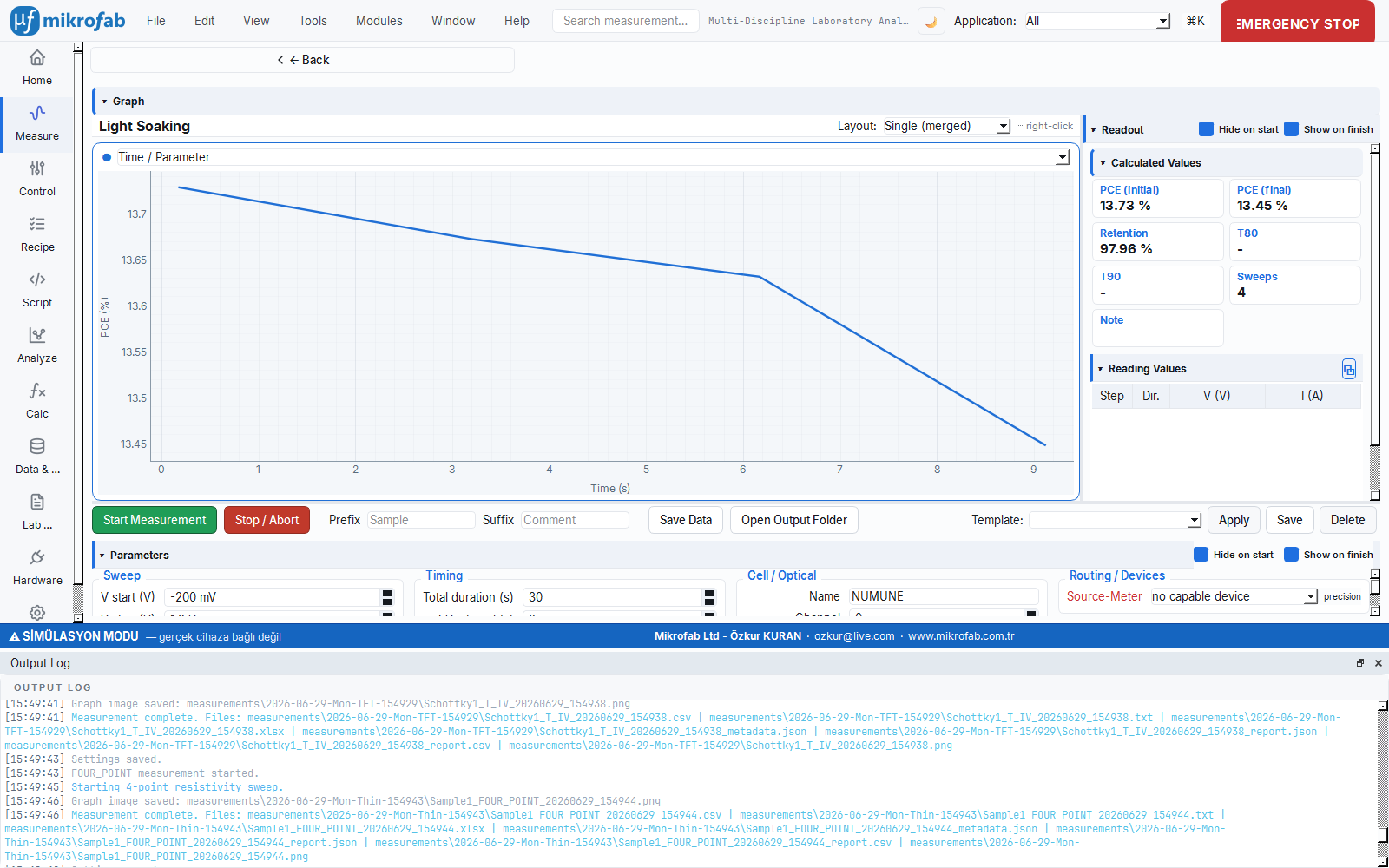
mppt_analysis module; a stability and efficiency summary from the tracking data.8.8 Light Soaking (pvsoak — measure.pv.soak)
It holds the cell under constant light for a long time, measures J-V at fixed intervals, and tracks how the efficiency changes over time. Like wearing a new shoe for days and observing how it settles in (or wears out), it reveals the effect of light exposure.
Physical background: Under continuous illumination, slow processes work in the cell: filling/emptying of traps, ion redistribution, and interface and metastable defect changes. These can initially increase the PCE (light-induced healing/activation) or gradually decrease it (degradation). The shape of the PCE(time) curve is the net result of these competing processes; T80/T90 are lifetime indicators that measure how long it takes for the efficiency to drop to 80%/90% of its initial value.
- Why it is done: to measure whether the cell heals or degrades under light, and how long it lasts.
- What it teaches / measures:
pce_initial/final_pct= the initial/final efficiency;retention_pct= 100·final/initial (the fraction of efficiency retained);t80_s/t90_s= the time at which the efficiency first drops to 80%/90% of its initial value (lifetime metrics, linear interpolation). - Typical values and interpretation: retention ≈ 100% (even >100% with light-induced healing) is stable/good; if retention is low or T80 is short, there is rapid degradation; never reaching T80/T90 (None) means the efficiency was maintained throughout the test.
- Common mistakes / cautions: keeping the test too short and missing slow degradation; attributing retention to the material without controlling the temperature/atmosphere (humidity, O₂); choosing too sparse a J-V interval (jv_interval) and failing to sample the early transient behavior.
- Where it is used: in stability and lifetime tests and in comparing material durability.
Purpose. Periodic J-V under continuous illumination; from PCE(time) it extracts the retention relative to the start and the T80/T90 aging metrics.
Additional parameters.
| Parameter | Unit | Description | Default |
|---|---|---|---|
total_duration_s | s | Total soaking duration. | 30.0 |
jv_interval_s | s | J-V repeat interval. | 3.0 |
Computed metrics.
pce_initial_pct = PCE of the first J-V
pce_final_pct   = PCE of the last J-V
retention_pct   = 100 · pce_final / pce_initial
t80_s           = time at which PCE first drops to 80% of initial (linear interp)
t90_s = time at which PCE first drops to 90% of initialThe PCE(time) curve is used; the 80% and 90% levels of the initial PCE are marked as horizontal threshold lines.
- Step: From the initial value, two horizontal lines are drawn for
0.80·PCE0and0.90·PCE0. - Step: The point where these lines first cross the PCE curve is brought down to the time axis by extrapolation (linear interpolation).
- Result: The times read are
t80_sandt90_s;retention_pct = 100·PCE_final/PCE0. (§8.9 Degradation uses the same method with a longer duration/interval.)
Plot: ts (time → PCE). Hardware: source + meter + light.
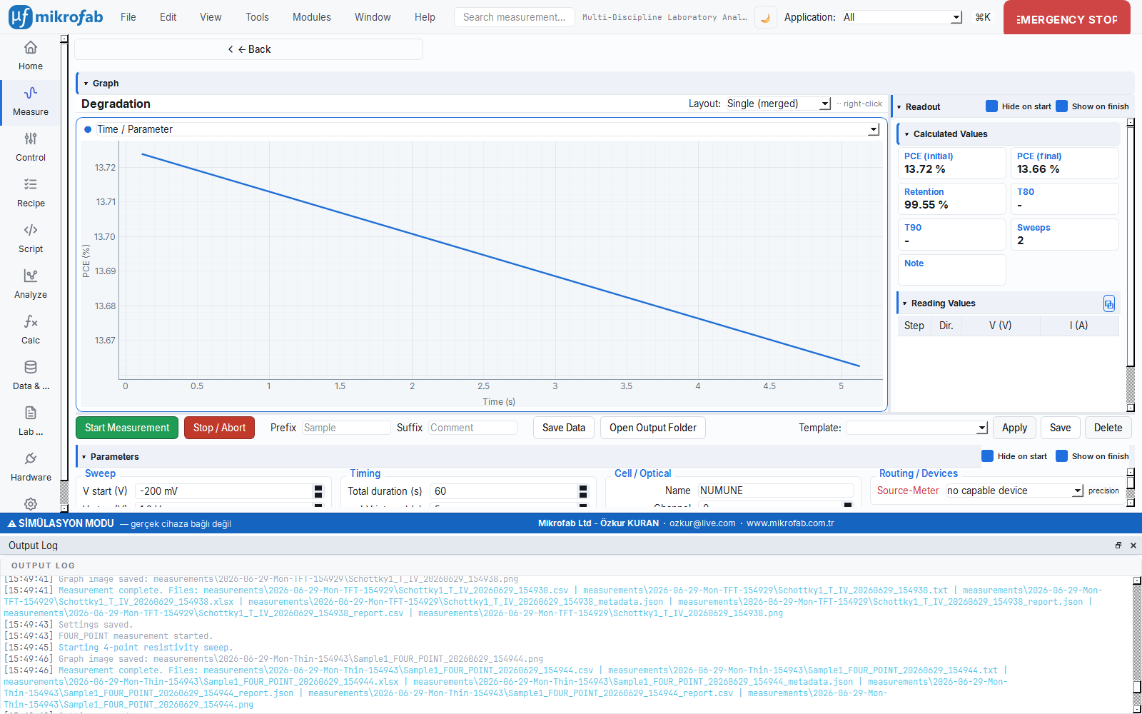
PCE(time), retention, and the T80/T90 aging metrics.8.9 Degradation (pvdegrad — measure.pv.degrad)
It works on the same logic as light soaking but tracks how the cell ages slowly over a longer time and at wider intervals. Like tracking the decline of a battery's charge-holding capacity over months, it records long-term degradation.
Physical background: Under prolonged stress, irreversible aging mechanisms accumulate: material decomposition, interface/contact deterioration, permanent trap formation, and moisture/oxygen-driven chemical change. Because these processes are slower than the reversible light-soaking transients, the measurement is done over a longer time and with sparser J-V; the PCE(time) curve generally shows a monotonically decreasing degradation trend.
- Why it is done: to quantitatively determine how long-lived the cell is in long-term use.
- What it teaches / measures: the same core as Light Soaking:
pce_initial/final,retention_pct,t80_s/t90_s(lifetime),n_sweeps(number of sweeps); the only difference is the longer default duration and interval. - Typical values and interpretation: a long T80 (a late-arriving 80% point) or retention staying high means good stability; a short T80 or rapidly falling retention means poor lifetime; remember that absolute times can be compared only under the same stress conditions (same light/temperature).
- Common mistakes / cautions: converting accelerated lab time directly to field lifetime (an acceleration factor is needed); sharing T80 without reporting the stress conditions (light, temperature, environment); taking the initial PCE from a point that has not yet settled (transient) biases retention.
- Where it is used: in reliability / durability tests and production quality assurance.
Purpose. It tracks parameter degradation over time and records the decline of the key metrics. It shares the same runner and metrics (PCE(t), retention, T80/T90) as Light Soaking; the difference is the longer default duration/interval.
Additional parameters. total_duration_s (default 60.0), jv_interval_s (default 5.0).
Computed metrics. Same as §8.8: pce_initial/final, retention_pct, t80_s, t90_s, n_sweeps. Plot: ts (time → PCE). Hardware: source + meter + light.
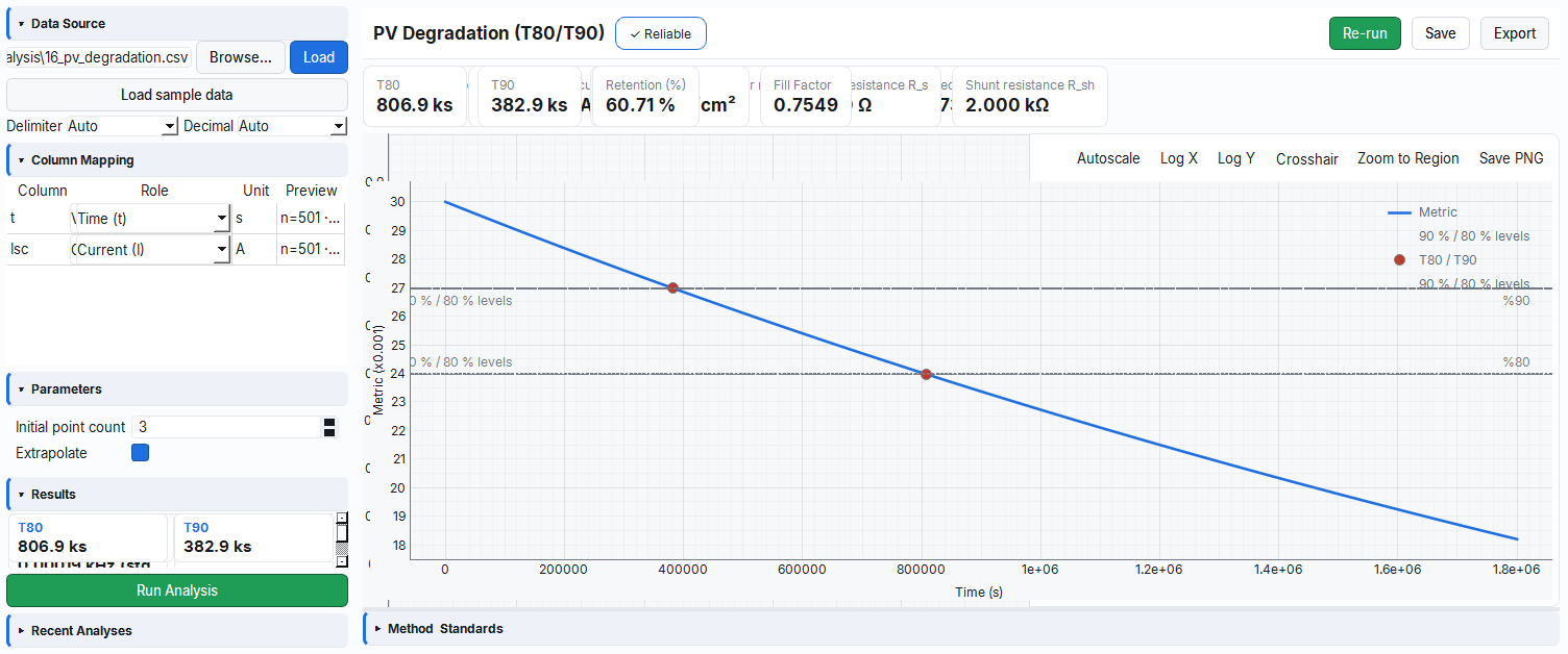
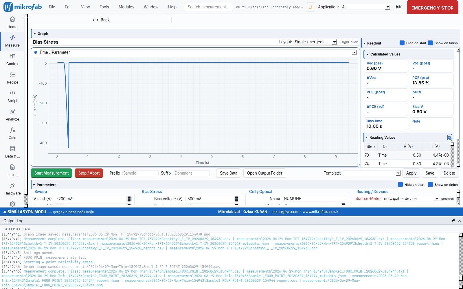
pv_degradation analysis module; retention and the T80/T90 aging metrics.8.10 Bias Stress (pvbias — measure.pv.bias_delta)
It first measures the cell's health (pre J-V), then holds it for a while at a given voltage (stress), and measures again afterward (post J-V). The difference between the two measurements shows what the biasing did to the cell; it is like inspecting a bridge for damage after holding a heavy load on it.
Physical background: Holding under a fixed bias forces the field and the carrier/ion distribution inside the cell: ions can migrate and accumulate at interfaces, traps can fill, and contacts can undergo electrochemical change. The I(t) recorded during the hold shows the "trace" of this slow rearrangement (increase/decrease); the difference between the pre and post J-V, meanwhile, reveals whether this stress left a reversible or a permanent change in performance.
- Why it is done: to measure whether electrical biasing degrades or improves the cell.
- What it teaches / measures:
delta_voc_v= the change in Voc;delta_pce_pct= the absolute change in PCE (percentage points);delta_pce_rel_pct= the relative (%) change in PCE; the direction of the I(t) slope during the hold (slow process) and, viabias_voltage/bias_duration_s, their dependence on voltage/duration. - Typical values and interpretation: Δ's ≈ 0 is a stable device (unaffected by biasing); a negative ΔPCE indicates bias-induced degradation, a positive ΔPCE indicates healing/activation; the Δ growing with longer duration points to slow ionic/trap processes.
- Common mistakes / cautions: measuring the pre/post J-V under different conditions (heated/cooled, different light) and attributing the Δ to stress; mistaking a reversible change (which reverts upon waiting) for permanent degradation; overlooking that the illumination state is assumed constant (the module does not drive light).
- Where it is used: in stability-mechanism research and operating-condition durability tests.
Purpose. A pre J-V → bias hold → post J-V sequence; it reports the bias-induced change in performance (degradation/improvement).
Additional parameters.
| Parameter | Unit | Description | Default |
|---|---|---|---|
bias_voltage | V | Voltage applied during the hold. | 0.5 |
bias_duration_s | s | Hold duration. | 10.0 |
bias_sample_interval_s | s | I(t) sampling interval during the hold. | 1.0 |
do_pre_jv | — | Whether to measure a pre J-V. | on |
do_post_jv | — | Whether to measure a post J-V. | on |
Computed metrics.
delta_voc_v       = Voc_post − Voc_pre
delta_pce_pct     = PCE_post − PCE_pre            (absolute; percentage points)
delta_pce_rel_pct = 100 · (PCE_post − PCE_pre)/PCE_pre   (relative %)
Hardware: source + meter (no light needed — constant external illumination is assumed). Plot: ts (during the hold, time → current, mA).
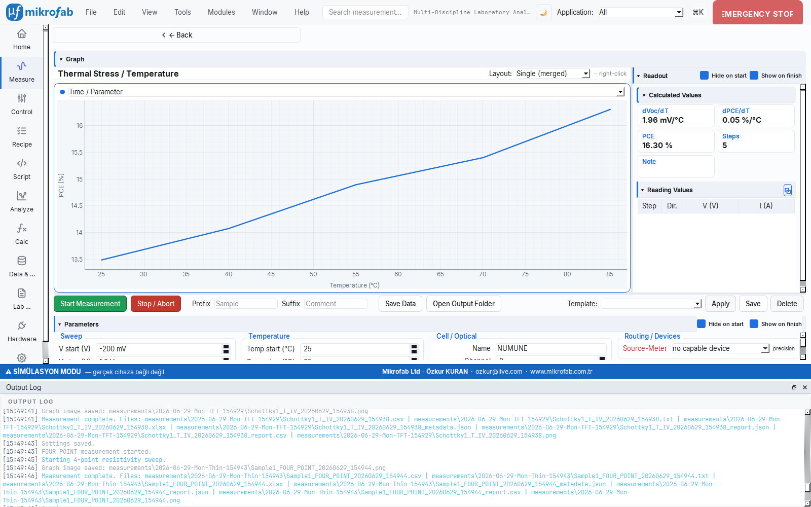
8.11 Thermal Stress / Temperature (pvthermal — measure.pv.thermal)
It brings the cell to different temperatures, measures a J-V at each, and extracts how performance changes with temperature. Solar panels heat up in the field; like testing whether a phone slows down when hot, it lets you predict behavior under real conditions.
Physical background: As temperature increases, the semiconductor's bandgap narrows slightly and the diode saturation current J0 grows exponentially; this notably lowers Voc (the dominant effect). Jsc increases very slightly because of the bandgap narrowing. The net result is that PCE decreases with temperature. The slopes of Voc and PCE versus temperature (dVoc/dT, dPCE/dT) summarize this behavior in a single number — these are generally negative.
- Why it is done: to know in advance how much efficiency the cell will lose on a hot panel in summer.
- What it teaches / measures:
dvoc_dt_mv_per_c= the temperature coefficient of Voc (mV/°C, depends on J0 and recombination);dpce_dt_per_c= the temperature coefficient of efficiency (%/°C);pce_final_pct= the efficiency at the highest temperature. - Typical values and interpretation: both coefficients are negative; in a silicon cell dVoc/dT ≈ −2 mV/°C and the efficiency drops measurably with temperature (relative ~0.3-0.5%/°C). A less negative coefficient means a cell that is more robust when hot (better for the field).
- Common mistakes / cautions: mistaking the controller's set temperature for the cell temperature (sufficient waiting is required for thermal equilibrium); deriving the slope (coefficient) from too few temperature steps; forgetting that this mode requires a temperature role on its own and that the sign of the slope (negative) is expected.
- Where it is used: in field-performance prediction and module design/rating.
Purpose. The J-V family at temperature steps; it extracts the temperature coefficients (dVoc/dT, dPCE/dT).
Additional parameters.
| Parameter | Unit | Description | Default |
|---|---|---|---|
temp_start_c | °C | Start temperature. | 25.0 |
temp_stop_c | °C | Stop temperature. | 85.0 |
temp_step_c | °C | Temperature step (a decreasing sweep is also supported). | 15.0 |
Computed metrics.
dvoc_dt_mv_per_c = (Voc–T slope) · 1000   [mV/°C]
dpce_dt_per_c    = PCE–T slope             [%/°C]
pce_final_pct = PCE at the last temperatureThe Voc (and PCE) extracted from the J-V at each temperature step is plotted against temperature (T); the points form an approximate line.
- Step: A least-squares line fit is performed separately on the
(T, Voc)and(T, PCE)points, and the slope of each is taken. - Result:
dvoc_dt_mv_per_c = (Voc–T slope)·1000[mV/°C],dpce_dt_per_c = PCE–T slope[%/°C]. Both slopes are typically negative.
Hardware: source + meter + light + temperature controller (the only PV mode that requires a temperature role). In mock, each temperature step changes the thermal voltage (kT/q). Plot: ts (temperature → PCE).
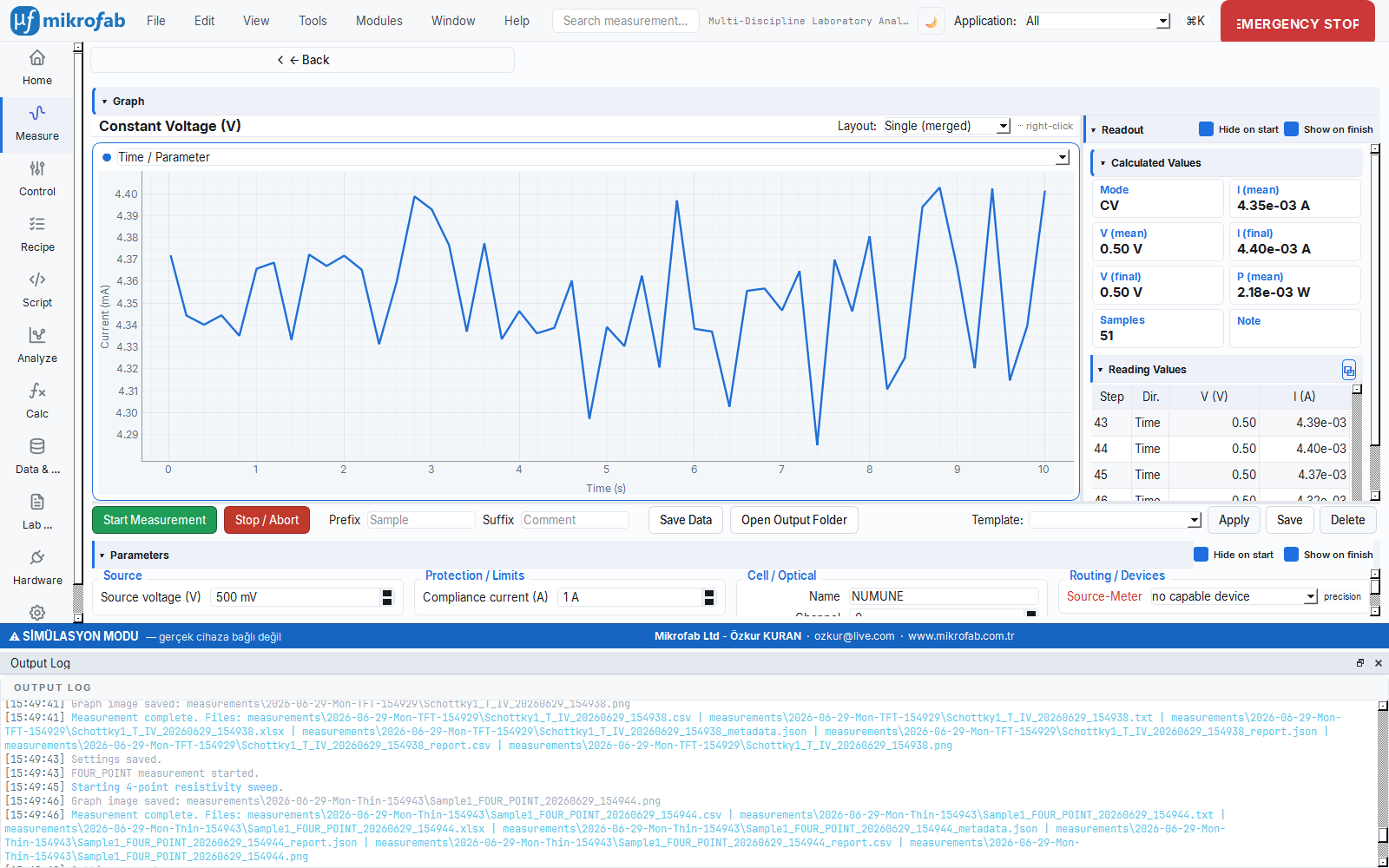
8.12 Constant Voltage — CV (pvcv — measure.pv.cv)
It holds a single voltage constant and records how the current settles (or drifts) over time. Like opening a tap to a fixed position and watching whether the water flow stabilizes, it shows the cell's stability at that point.
Physical background: When the voltage is held constant, the slow change in the current reveals the transient processes inside the cell: discharge of capacitive charge, trap filling/emptying, ion redistribution, and thermal settling. In an ideal stable cell I(t) quickly settles to a horizontal value; a continuously drifting or slowly settling current indicates an internal dynamic (e.g. ionic) that responds to voltage with a lag.
- Why it is done: to observe whether the current is stable at a particular operating point.
- What it teaches / measures:
i_mean_a/i_final_a= the mean/final current;v_mean_v/v_final_v= confirmation of the applied voltage;p_mean_w= mean(V·I) power;n_samples= the number of samples; and the settling behavior of the I(t) curve. - Typical values and interpretation: i_final ≈ i_mean and a flat I(t) indicate stable operation; a current that peaks at the start and decays indicates capacitive/transient discharge, while a continuously drifting current indicates an unsettled (unstable) point.
- Common mistakes / cautions: keeping the total duration shorter than the settling time constant and mistaking a not-yet-settled current for "stable"; choosing too large a sampling interval and missing the early transient; choosing the applied voltage outside the protection/limit range.
- Where it is used: in stability checking, settling-time measurement, and simple durability trials.
Purpose. A constant voltage is applied and the current I(t) is recorded as a time series (stability / settling monitoring).
Additional parameters.
| Parameter | Unit | Description | Default |
|---|---|---|---|
source_voltage | V | Applied constant voltage. | 0.5 |
total_duration_s | s | Total duration. | 20.0 |
sample_interval_s | s | Sampling interval. | 0.2 |
Computed metrics. i_mean_a, v_mean_v, i_final_a, v_final_v, p_mean_w = mean(V·I), n_samples. Hardware: source + meter. Plot: ts (time → current, mA).
8.13 Constant Current — CI (pvci — measure.pv.ci)
This time the current is held constant and the change in voltage over time is tracked; it is the inverse of CV. Like pedaling at a constant speed and measuring how much power you expend, it forces the cell at a given current and observes its response.
Physical background: When a constant current is driven, the SMU continuously adjusts the voltage needed to pass that current; the slow change in V(t) shows how the cell's "difficulty" in carrying that current changes over time. An increasing series resistance, contact deterioration, or ion/trap redistribution can shift the voltage up/down. Depending on the current direction, the point corresponds to a different region of the J-V curve (generation or forward bias).
- Why it is done: to see whether the voltage stays stable when a constant current is drawn.
- What it teaches / measures: the same summary as CV —
v_mean_v/v_final_v= the mean/final voltage (the main interest);i_mean_a/i_final_a= confirmation of the driven current;p_mean_w= mean power;n_samples; and the V(t) drift behavior. - Typical values and interpretation: a flat V(t) indicates stable operation; a continuously rising voltage indicates increasing series resistance/contact deterioration, while fluctuation indicates an unstable internal dynamic.
- Common mistakes / cautions: the driven current exceeding the safety current limit causes the measurement to be rejected before it starts (
Kaynak akimi guvenlik limitinin uzerinde); also, at too high a current the voltage may hit the protection limit (voltage_limit) — the current should be chosen according to the cell's capacity. - Where it is used: in stability monitoring and current-driven operation trials.
Purpose. A constant current is driven and the voltage V(t) is recorded as a time series.
Additional parameters.
| Parameter | Unit | Description | Default |
|---|---|---|---|
source_current | A | Driven constant current. | 0.001 |
total_duration_s | s | Total duration. | 20.0 |
sample_interval_s | s | Sampling interval. | 0.2 |
Computed metrics. The same summary as CV (i_mean/v_mean/i_final/v_final/p_mean/n). Hardware: source + meter + light.
Kaynak akimi guvenlik limitinin uzerinde).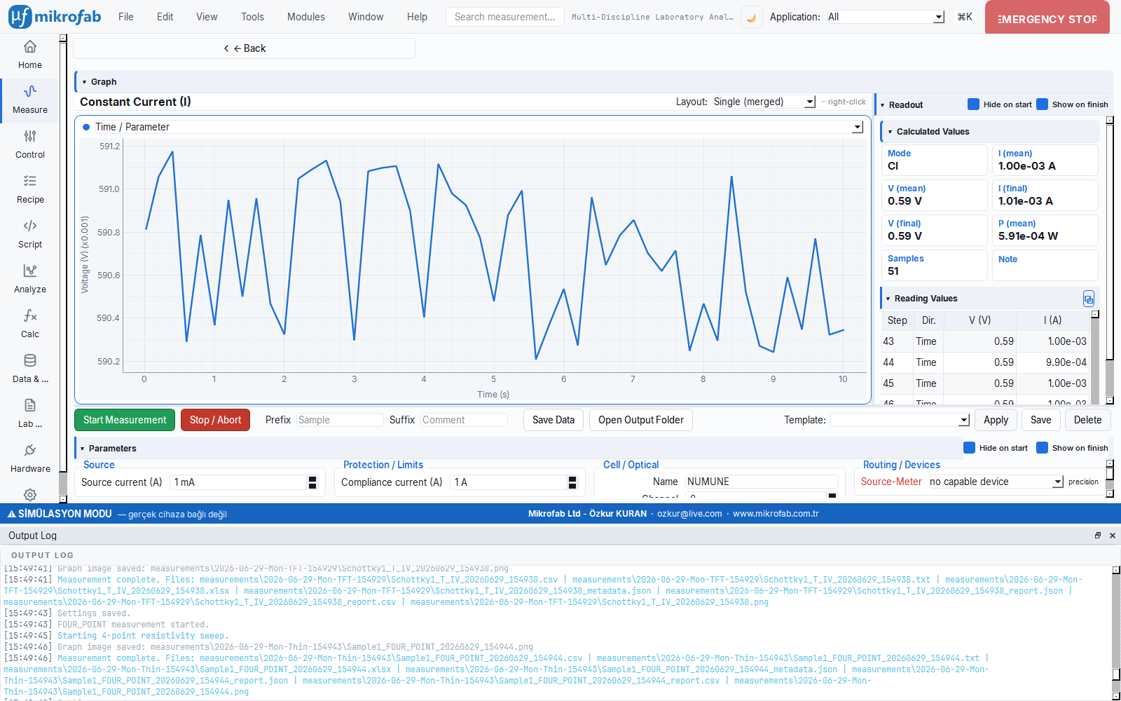
8.14 Multi-cell Batch / ChannelGrid (pvgrid — measure.pv_grid)
It automatically selects, one by one, many cells placed in a switching fixture and measures them in sequence. Like automatically grading the exams of an entire class and producing a transcript, it produces batch results and statistics without manual effort.
Physical background: A switch (relay) matrix connects the same SMU in turn to the contacts of different cells; an independent PV J-V is measured for each cell and the same metrics are extracted from the single-source core. The spread of PCE from cell to cell (mean ± std) shows the fixture/process uniformity; spatial patterns in the PCE heatmap (e.g. low edges) reveal systematic variation caused by coating/process.
- Why it is done: to measure and compare many cells quickly, consistently, and without human error.
- What it teaches / measures: per-cell PCE (color/heatmap), overlaid J-V curves, and batch statistics: mean ± std (n) for PCE/Voc/FF/Jsc (
summarize_batch, single source); the size of the std measures the repeatability. - Typical values and interpretation: a small std (narrow distribution) means high production uniformity; a wide distribution or a spatial gradient in the heatmap indicates a process/coating problem; gray (unmeasured) cells indicate a faulty selection/contact.
- Common mistakes / cautions: an unvalidated relay map does not send commands on real hardware (only mock/grid) — failing to notice this; not entering the area/irradiance correctly for all cells biases the statistics; one cell's error does not stop the others (
ok=Falserecord), so overlooking this and mistaking incomplete data for complete. - Where it is used: in production-line screening, quality control, and screening large sample sets.
Purpose. On a switched fixture grid (38/22/20/10 relay map) it measures multiple cells in sequence with PV J-V; it extracts a PCE heatmap across cells and batch statistics.
Flow.
- A relay map is selected (
pv_relay_map; an unvalidated map does not send commands on real hardware — only mock/grid). - With Run Batch, each cell is selected in turn (
select_cell), a PV J-V is measured (PVJvMeasurementRunner), and thePVJvSummaryis collected. - The cells are colored by PCE (unmeasured = gray); there is also an overlaid J-V curves view (with the cell's color).
- Batch statistics: mean ± std (n) for PCE / Voc / FF / Jsc (
summarize_batch, single source). The results are exported to CSV.
Parameters. The same fields as single-cell PV J-V (sweep direction default Forward; area 1 cm²; irradiance 1000 W/m²). Hardware: source + meter + switch matrix + light.
Safety. Because switching is done externally, no relay is given to the runner (no double-selection); one cell's error does not stop the others (ok=False + error record), and at the end of the batch the relays are turned off with all_off.
9. Screenshot Mapping (Summary)
| nav_key | Screenshot path |
|---|---|
pvws | assets/screenshots/meas_pvws.png |
pvdarkjv | assets/screenshots/meas_pvdarkjv.png |
pvhyst | assets/screenshots/meas_pvhyst.png |
pvpulsed | assets/screenshots/meas_pvpulsed.png |
pvsunsvoc | assets/screenshots/meas_pvsunsvoc.png |
pvintensity | assets/screenshots/meas_pvintensity.png |
pvmpp | assets/screenshots/meas_pvmpp.png |
pvsoak | assets/screenshots/meas_pvsoak.png |
pvbias | assets/screenshots/meas_pvbias.png |
pvdegrad | assets/screenshots/meas_pvdegrad.png |
pvthermal | assets/screenshots/meas_pvthermal.png |
pvcv | assets/screenshots/meas_pvcv.png |
pvci | assets/screenshots/meas_pvci.png |
pvgrid | assets/screenshots/meas_pvgrid.png |
pv_metrics, pv_hysteresis, and pv_diode modules in the Analysis workspace; you can later load the measured data and re-verify the same metrics (see the Analysis Modules — Photovoltaic section).